Chapter 9: Correlation, diversification, and factor tilts
What diversification actually is, one cell of the correlation matrix at a time, why forty holdings can carry the risk of one, and the factor lens that identifies the bet.
By Matt Lang and Bree Lang · About the authors
Where this is on Sifter: Portfolio · Analyze · Diagnostics
Imagine that the Maple Fund's investment committee is feeling rather pleased with itself. The book holds three active stocks in three different sectors (MPL in technology, BRC in healthcare and CDR in energy), and if you asked any member of the committee whether the fund was diversified, they would point at the three sector labels and say yes. Now take a minute and look at the table below, which lists what each of the three stocks did on each of the ten trading days we have been using since Chapter 3. On the days MPL went up, BRC went up. On the two days MPL fell, BRC fell with it. CDR, meanwhile, spent the two weeks wandering around on its own schedule, up on days the other two were down and down on days they were up. In other words, two of the three stocks have been behaving like one position that happens to wear two tickers, which means that the committee owns fewer independent bets than the sector labels suggest.
So how much diversification does the fund actually have? Sector labels cannot answer that question, because a sector label describes what a company sells, and the only thing that matters for the risk of a book is how its stocks move. Statisticians measure how much two series move together with the correlation coefficient, a number that runs from +1 (the two move in lockstep) through 0 (no relationship at all) to −1 (they move in opposite directions). This may seem like a simple definition, but there is a lot to it. The Diagnostics tab draws a whole grid of these numbers, one for every pair of holdings in the book, and calls the grid the correlation matrix. In this chapter we will build one cell of that grid by hand, read the whole grid, and then work out what the number does to the risk of a portfolio, which is the reason anyone bothers to diversify in the first place. Once we have done that, we will turn a second Diagnostics panel, the factor card, on the same book, because the matrix can find a hidden bet but it takes the factor lens to say what the bet is.
Maple Fund: daily returns by stock
| Day | Date | MPL | BRC | CDR |
|---|---|---|---|---|
| 1 | 2026-01-05 | 1.5% | 0.8% | -1.4% |
| 2 | 2026-01-06 | -0.8% | -0.6% | -0.3% |
| 3 | 2026-01-07 | 0.4% | 0.6% | -0.5% |
| 4 | 2026-01-08 | 0.1% | 0.1% | -1.3% |
| 5 | 2026-01-09 | 1.2% | 0.4% | 0.5% |
| 6 | 2026-01-12 | 1.6% | 1.6% | -0.6% |
| 7 | 2026-01-13 | -0.6% | 0.1% | -0.4% |
| 8 | 2026-01-14 | 0.7% | 1.0% | 0.7% |
| 9 | 2026-01-15 | 0.2% | 0.4% | 0.8% |
| 10 | 2026-01-16 | 0.9% | 0.4% | -0.4% |
Like the sector table in Chapter 8, this is a period-level view of the Maple Fund with its own numbers, so do not expect the three columns to average back to the fund's daily returns from Chapter 3. Before doing any arithmetic, run your eye down the MPL and BRC columns together and count how many days they share a sign. Then do the same for MPL and CDR. You already know what the matrix is going to say.
One cell of the matrix
Before we compute anything, let's be clear about what we are computing. The correlation matrix is a grid with one row and one column for every holding, and each cell holds a single number, the correlation between the holding in that row and the holding in that column. For the Maple Fund's three stocks that is a three-by-three grid, and because the correlation of MPL with BRC is the same number as the correlation of BRC with MPL, and every stock's correlation with itself is exactly one, the grid really only contains three numbers worth computing. We are going to compute one of them, the MPL and BRC cell, from the ten daily returns in the table above, and the formula below is the recipe. It looks busier than it is. The top of the fraction asks whether the two stocks tend to be above or below their own averages on the same days, and the bottom of the fraction scales the answer so that it lands between −1 and +1.
Correlation
r_A and r_B are the two stocks' daily return series. Cov is their sample covariance, the average product of the two series' deviations from their own means, divided by n − 1 in the same way as the sample standard deviation from Chapter 5. The two σ are the sample standard deviations of the same two series. Dividing by both standard deviations strips the units away, so ρ is a pure number between −1 and +1 no matter how volatile either stock happens to be. The platform computes it on simple daily returns (close over prior close, minus one) over the trailing twelve months.
Worked example: Worked example: the MPL and BRC cell
Let's build one cell of the matrix from scratch, because once you have done it for one pair you have done it for every pair. We will take MPL and BRC, the two stocks that looked like twins in the table.
- Find each stock's mean daily return MPL: add the ten returns (1.5%, -0.8%, 0.4%, 0.1%, 1.2%, 1.6%, -0.6%, 0.7%, 0.2%, 0.9%) and divide by 10 = 0.52%. BRC: the same over its column = 0.48%. MPL averaged 0.52% a day over the two weeks and BRC averaged 0.48%. Both means are small, which is normal for daily returns, and the sign of the mean has nothing to do with what comes next.
- Subtract the means to get each day's deviation MPL deviations: 0.98%, -1.32%, -0.12%, -0.42%, 0.68%, 1.08%, -1.12%, 0.18%, -0.32%, 0.38%. BRC deviations: 0.32%, -1.08%, 0.12%, -0.38%, -0.08%, 1.12%, -0.38%, 0.52%, -0.08%, -0.08%. Take a moment to compare the two rows sign by sign. On nearly every day the two deviations share a sign, which means that when MPL was above its own average, BRC was above its average too. That shared sign is the whole idea, and the next step just turns it into a number.
- Multiply the deviations day by day, then add them up Products, in percent squared (multiply each decimal product by 10,000): 0.31, 1.43, -0.01, 0.16, -0.05, 1.21, 0.43, 0.09, 0.03, -0.03. Sum = 3.55. A day where both deviations are positive gives a positive product, a day where both are negative also gives a positive product (two negatives), and only a day where the two disagree subtracts from the pile. The sum is comfortably positive here because the disagreements were few and small.
- Divide by n − 1 to get the covariance Cov = 3.55 / 9 = 0.395 percent squared (which is 3.949e-5 in decimals). The covariance has the right sign and the arithmetic is straightforward, but the number is nearly impossible to interpret on its own, because its units are a percent multiplied by a percent, and nobody has any intuition for a squared percent. In order to turn it into something readable we scale it by the two standard deviations in the last step.
- Divide by both standard deviations σ_MPL = 0.820%, σ_BRC = 0.588% (STDEV.S over each column). ρ = 0.395 / (0.820 × 0.588) = 0.395 / 0.483 = 0.82. The correlation between MPL and BRC over the two weeks is 0.82. Take a moment to think about what that number means. On a scale where +1 is two stocks moving as one and 0 is two stocks ignoring each other, these two are most of the way toward moving as one, which is exactly what your eye told you from the table. The number just lets you say it precisely, and lets the platform say it for every pair in a fifty-stock book without anyone's eyes getting involved.
The Maple Fund correlation matrix
| MPL | BRC | CDR | |
|---|---|---|---|
| MPL | 1.00 | 0.82 | -0.09 |
| BRC | 0.82 | 1.00 | 0.02 |
| CDR | -0.09 | 0.02 | 1.00 |
The other two cells were computed the same way. The diagonal is 1.00 by definition, since every stock moves in perfect lockstep with itself, and the matrix is symmetric, since the correlation of MPL with BRC is the same number as the correlation of BRC with MPL. This means that a matrix of N stocks contains only N(N − 1)/2 distinct numbers, which for three stocks is three and for the twelve stocks on the platform's default view is sixty-six.
Reading the whole grid
Now that we have the matrix, let's read it the way the committee should have. MPL and BRC are at 0.82, which is the twins. MPL and CDR are at -0.09 and BRC and CDR at 0.02, both of which are close enough to zero that, over these two weeks, CDR had essentially nothing to do with the other two. So the fund does own two independent bets after all, but it owns two and not three, and the bigger of the two (MPL plus BRC together) is 60% plus 25% of the book. The sector labels said three bets of 60%, 25% and 15%. The matrix says one bet of 85% and one of 15%, and a committee that knows the second description is going to run the fund differently from one that only knows the first.
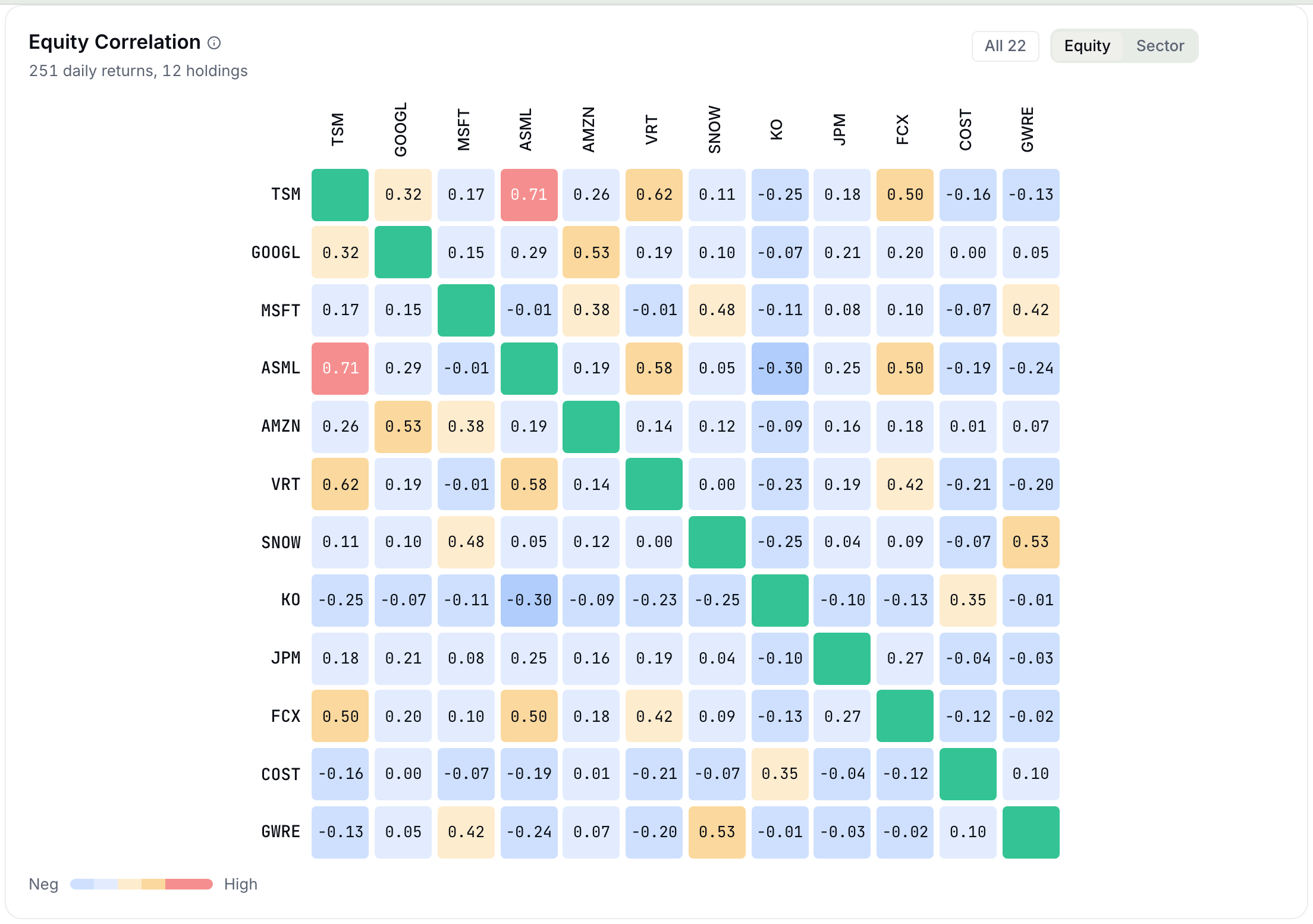
On your own book the panel is on Portfolio › Analyze › Diagnostics, directly under the tab header, and the way it is built affects how you read it. The platform takes the twelve largest holdings by value (a button switches to the full book), leaves out cash and the index funds, pulls a year of daily prices for each holding, and computes the correlation of every pair over the trading days the two stocks have in common. A pair needs at least ten days in common and the whole grid needs at least twenty, and a pair that cannot be measured (a stock listed last week, say) shows a small dot in its cell rather than a number, because printing a made-up number in a grid of measured ones gets a fund into trouble. Cells are shaded so that the warm colors mark pairs above about 0.5 and the deep red marks pairs above 0.7, which means that you can read a fifty-stock matrix from across the room and see where the twins are. Hover a cell and the panel prints the number to three decimals along with a sentence saying what it means. The figure below is the panel on a real fund's book.
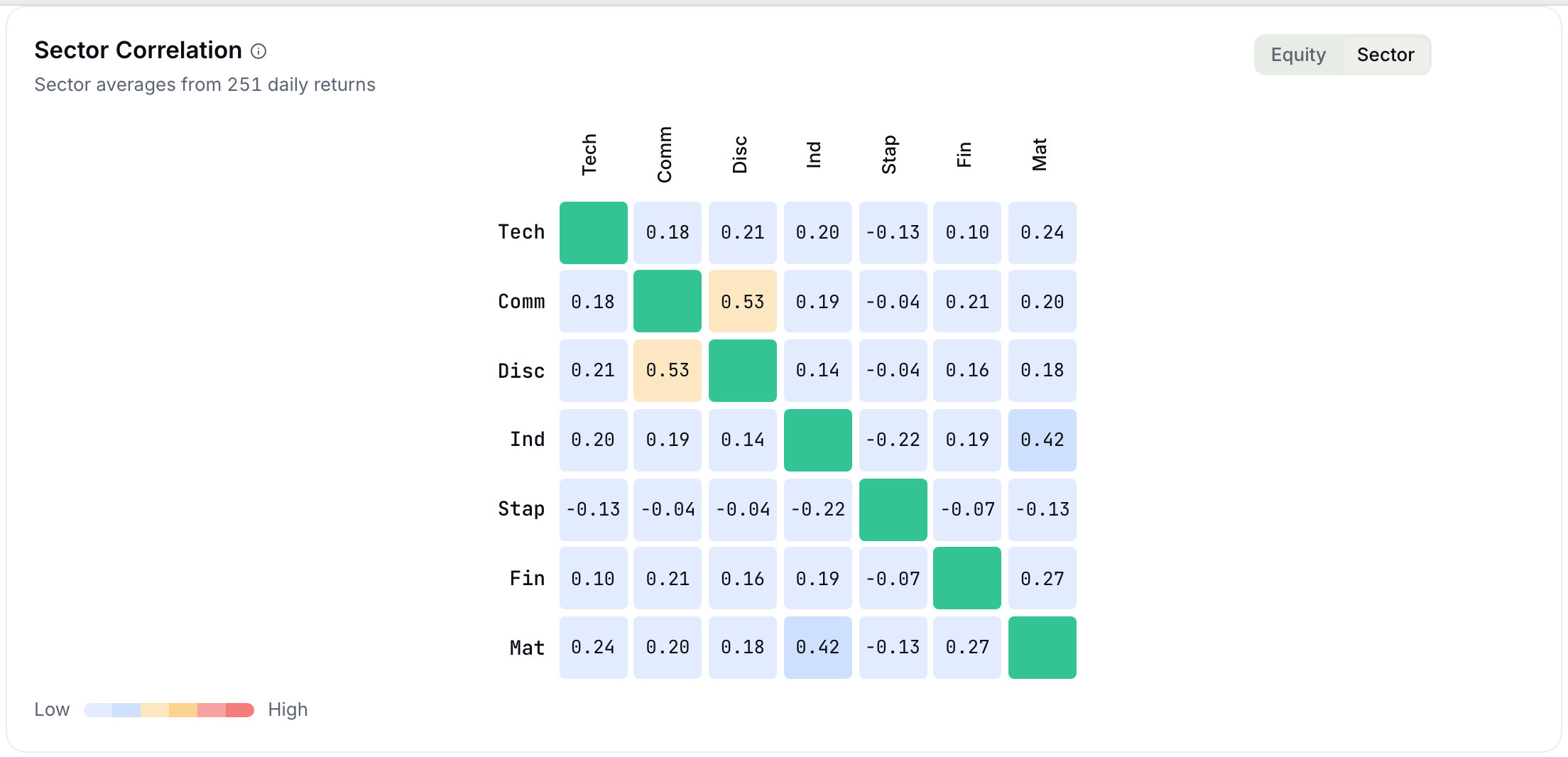
The same panel has a second view, labeled Sector, which folds the stock-by-stock numbers up into sector-by-sector averages. Each cell of the sector view is the average of the measured correlations between every stock in one sector and every stock in another, so it is built from the same year of returns rather than from a lookup table (the platform only falls back to a table of long-run sector estimates when a book has no price history yet, and it says so in the subtitle when it does). The sector view is the right one to bring to a committee meeting, since it answers the question the committee is actually asking, which is whether the fund's technology holdings and its industrial holdings are two bets or one. The stock view is the right one for a portfolio manager deciding what to buy next. The figure below is the same book folded into sectors.
What correlation does to a book
Portfolio variance, two stocks
w_A and w_B are the two weights (they sum to one), σ_A and σ_B are the two stocks' volatilities from Chapter 5, and ρ_AB is the correlation we just built. The first two terms are what each stock contributes on its own. The third term is the one this chapter is about, because it is the only place the correlation enters, and it can be large and positive, zero, or negative. With more than two stocks the formula grows a term for every pair, w_i w_j ρ_ij σ_i σ_j, which is why the platform needs the whole matrix and not just a list of volatilities.
Take a minute to look at that third term, because it is the reason diversification works when it works and fails when it fails. If the correlation is zero the term vanishes, and the book's variance is just the two weighted variances added together, which is already less than either stock's variance alone because the weights get squared (half of a stock, squared, is a quarter of its variance). If the correlation is +1 the term is as large as it can be, and the formula collapses to (w_Aσ_A + w_Bσ_B)², which means that the book's volatility is just the weighted average of the two volatilities and owning both stocks bought you nothing. Every real pair falls somewhere between those two cases, and where it falls is the correlation.
This also settles a question that comes up at nearly every student fund at some point, which is whether more holdings means more diversification. Imagine a book of N stocks, all with the same volatility σ, all held at equal weight, and all correlated with each other at the same ρ. Working through the formula (there are N variance terms and N(N − 1) covariance terms) gives a portfolio variance of σ² × (1/N + ρ(N − 1)/N). The first piece, 1/N, is the part that diversifying away can remove, and it shrinks toward zero as you add holdings. The second piece does not shrink at all. As N grows the whole expression heads toward ρσ², which means that the risk you cannot diversify away is set entirely by the average correlation between your holdings.1 Let's put numbers on it. Forty holdings at a correlation of 0.8 carry about 90% of a single stock's volatility, and eight holdings at a correlation of 0.2 carry about 55%. In other words, the eight-stock book is the better-diversified one by a wide margin, and a fund that adds its twentieth technology stock in the belief that it is spreading risk is mostly adding paperwork.
Practice
Build an equal-weighted book of just MPL and BRC. Using the annualized volatilities from the Maple table (MPL 13.0%, BRC 9.3%, both from the ten-day standard deviations times √252), what would the book's annualized volatility be if the two stocks were uncorrelated (ρ = 0)? Answer in percent.
Solution. σ²_p = 0.25 × 13.0%² + 0.25 × 9.3%² = 0.25 × 169.6 + 0.25 × 87.2 = 64.2, so σ_p = √64.2 = 8.0%. Notice that this is below both stocks' own volatilities, and well below their simple average of 11.2%. That difference is what two uncorrelated stocks buy you, and it is the diversification the committee thought it had.
Practice
Now put the covariance term back. With the measured correlation of 0.82 between MPL and BRC, what is the same equal-weighted book's annualized volatility? Answer in percent.
Solution. The covariance term is 2 × 0.5 × 0.5 × 0.82 × 13.0% × 9.3% = 49.8, so σ²_p = 64.2 + 49.8 = 114.0 and σ_p = 10.7%. Take a moment to compare the two answers. The uncorrelated version of this book ran at 8.0% and the real one runs at 10.7%, which is most of the way back toward the simple average of the two volatilities. This means that owning both MPL and BRC removed only a small slice of the risk of owning either one, and the reason is the 0.82 and nothing else.
Correlated clusters
The platform uses the matrix one more way, and it is the way a fund's risk limits are written. Rather than asking about pairs, it asks about groups. Take every pair whose correlation is at or above some line (the default line is 0.60), draw a link between the two holdings, and then collect every holding that is connected to every other by some chain of links. Each connected group is a correlated cluster, and its size is measured as the combined weight of its members. The chain rule matters more than it looks. If A is linked to B and B is linked to C, then A and C land in the same cluster even when A and C themselves are at 0.3, because the cluster is asking a different question from the pair. The pair asks whether two stocks move together. The cluster asks how much of the book moves together in a bad week, and a bad week travels along the chain.
On the Maple Fund the arithmetic is short. MPL and BRC are at 0.82, which is above the 0.60 line, so they are linked. CDR is below the line against both, so it stands alone. The fund therefore has one cluster, MPL and BRC, and its weight is 60% plus 25% using the weights from the sector table in Chapter 8. Risk Flags on a fund's Portfolio shows the same clustering for the real book, using the full matrix over the trailing year, and it prints two numbers from it next to the fund's limits. The first is the largest cluster's weight, and the second is the single highest pairwise correlation in the book (the default line for that one is 0.70). We will come back to what a fund does with those two numbers in Chapter 21, when we get to risk limits. For now the point is that both of them are read straight off the matrix you just built.
Practice
Using the Maple matrix and a cluster line of 0.60, what is the combined weight of the largest correlated cluster, as a percent of the book?
Solution. Only one pair clears the line, MPL and BRC at 0.82. Their weights are 60% and 25%, so the cluster is 85% of the book. Take a moment to think about what that means for a fund that believed it held three sector bets. In a week when technology and healthcare sell off together, 85% of the Maple Fund is going the same direction at once, and only CDR's 15% is doing anything else. A real fund's risk limits typically cap a cluster at something like a quarter of the book, which gives you a sense of how far this three-stock example is from a diversified one.
Check yourself
Two holdings on your book show a correlation of 0.90 over the trailing year. Which of the following statements does that number actually support?
- The two companies are in the same industry. Not necessarily. Correlation measures how the two stocks moved, not why. Two companies in different industries can share a customer, a currency, a commodity price or simply a crowd of the same investors, and any of those will produce a 0.90. The number tells you to go and find out why, and it does not tell you the answer.
- Over the past year the two moved up and down together on most days, so for the book's risk they behaved like one larger position. (correct) Right. That is what the number says, and it is enough to act on. A 0.90 pair adds almost its full covariance term to the book's variance, so for sizing and for the cluster arithmetic the two holdings are close to one position with their weights combined.
- The two will keep moving together next year. The matrix is measured over a window that has already happened, and correlations change, sometimes quickly. A 0.90 over the past year is a good reason to expect the two to stay related, but it is not a promise, and a fund that treats a measured correlation as a law is going to be surprised at the worst possible time.
- Owning both was a mistake. The number is a measurement, not a verdict. A fund can hold a 0.90 pair on purpose (two ways of expressing one strong view, sized together), and the matrix is there so that the committee knows it is doing so. What the number rules out is holding both and believing they are two separate bets.
Rebuild a cell on your own book
Lab: CSV lab: rebuild one cell of the matrix
- On Portfolio › Analyze › Diagnostics, download the Verify CSV. The same file you used in Chapter 7 now has three correlation sections, CORRELATION METHOD, CORRELATION MATRIX (equity) and CORRELATION DAILY RETURNS (decimal).
- In the CORRELATION DAILY RETURNS section, every column after Date is one holding's daily return series over the trading days all of them share. Pick any two columns.
- Run CORREL() over the two columns (or build it the long way with the worked example above, which takes about a minute in a spreadsheet).
- Find the same pair in the CORRELATION MATRIX section and compare. The two should agree to the fourth decimal, because the platform computed its cell from exactly the rows you just used.
The factor lens
The matrix tells you that two holdings have been moving together, and it leaves you to work out why. Sometimes the reason is obvious (two regional banks, say), but the Maple Fund's twins are in different sectors, and a fund that wants to know what it is actually betting on needs a second lens. Imagine that you ask a portfolio manager to describe her fund. If she is a stock picker, she will do what stock pickers have always done and walk you through the book one company at a time. A risk model describes the same portfolio in a much blunter way. To the model, the book is a bundle of styles, and the only things worth knowing are how small, how cheap, how recently strong and how profitable the holdings are compared to the market. These comparisons are called factor tilts, and they matter because factors, not tickers, explain most of why diversified portfolios move together. Take a fund that proudly holds "twelve unrelated companies," every one of them an expensive mega-cap growth stock. The matrix would show you the twelve moving together, and the factor panel would tell you the reason, which is that the fund holds one bet twelve times over. In other words, the two panels answer the same question from opposite ends. The matrix finds the twins after the fact, and the factor panel identifies the common bet that made them twins.
Sifter shows factors in two places, and the two are easy to confuse. The Factor Tilts card under Analyze › Diagnostics is holdings-based, which means that it scores what you own. Every holding in your book gets a number on each of five style factors from the company's own current characteristics (its market cap, its earnings yield and so on), and the numbers are rolled up to the book at portfolio weights. The Regression card next to it is return-based. It compares your book's daily returns to each factor's daily returns over time and reports a beta to each one, the same way Chapter 6 fitted a beta to the market. The two cards share factor names but measure different things, and this chapter spends its time on the holdings-based card because that is the one you can check by hand.
So what kind of number is a factor tilt? Every score on the holdings-based card is a z-score, a count of standard deviations. A holding's Size score of +1.0 says that the company is one standard deviation smaller than the market, a score of −2.0 says that it is two standard deviations larger, and most holdings land somewhere between −2 and +2, which means that a book, being an average of its holdings, usually lands within a few tenths of zero. The five factors are Size (SMB, small minus big), Value (HML, high minus low), Momentum (UMD, up minus down), Profitability (RMW, robust minus weak) and Investment (CMA, conservative minus aggressive), with a sixth, descriptive Low Volatility score shown alongside. Each score is measured against the S&P 500 constituents, a universe the platform refreshes every day, and the card has a "Holdings-based" badge so that you always know which of the two you are reading. (The market factor itself is not on this card. Beta is a return-based measure, and it appears on the Regression card and in the Risk Lab, where the platform regresses your daily returns on the six Fama-French series.) The codes probably look like alphabet soup at the moment, but each one is an abbreviation with a story behind it, and the callout below tells it.
The five factors
| Factor | Code | Spelled out | A positive tilt means | Measured by |
|---|---|---|---|---|
| Market | β | beta to the market | the book swings harder than the index | regression on market returns (Chapter 6's beta; on the Regression card, not this one) |
| Size | SMB | small minus big | behaves like smaller companies | log of market cap, sign flipped so that small scores positive |
| Value | HML | high minus low | tilted toward cheap stocks | earnings yield and book-to-price, each z-scored and then averaged |
| Momentum | UMD | up minus down | tilted toward recent winners | price 21 trading days ago over price 252 trading days ago, minus one |
| Profitability | RMW | robust minus weak | tilted toward high-profit firms | gross profit over assets |
| Investment | CMA | conservative minus aggressive | tilted toward firms that grow assets slowly | asset growth, low growth scoring conservative |
Take a closer look at the Momentum row before moving on, because it hides a wrinkle. The most recent month of returns tends to REVERSE (a short-term bounce-back), so the convention skips it and measures months 12 through 2, following the study that documented the effect over 3- to 12-month holding periods.4 The platform also computes a descriptive low-volatility score, but it stays out of the headline panel because low volatility is a characteristic rather than a priced Fama-French factor.
A factor exposure is a z-score
The mean is cap-weighted (the market's average), the dispersion equal-weighted, and extreme scores are clipped at ±3 so one wild data point cannot dominate. Value has two ingredients, so its z is the average of the two. A holding missing a characteristic takes its sector's median z and is marked with a dagger in the table, and a fund with no fundamentals at all is left out, with the card's coverage line saying how much of the weight was mapped. Portfolio exposure = weighted average of holding z-scores; ACTIVE exposure subtracts the benchmark's, which by construction is near zero. Active near zero on every factor while holding different stocks is the signature of pure stock-picking.
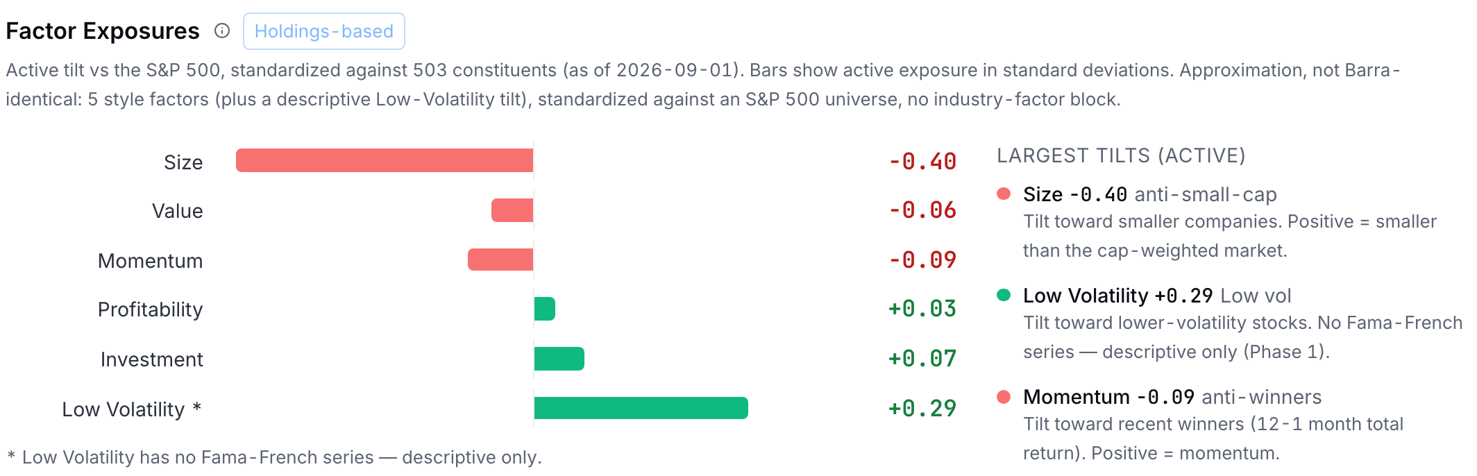
The figure below is the card on the sample book. Every bar is an active exposure in universe standard deviations, and the panel to its right lists the three largest. This particular book is four tenths of a standard deviation LARGER than the market on Size (the card says "anti-small-cap"), a touch behind on Momentum, and a little calmer than the index on the descriptive Low Volatility line, which is roughly what you would guess from a list of mega-cap stocks, and the point of the card is that you no longer have to guess.
Scoring one holding
Worked example: Worked example: scoring one holding on Value
Let's score one holding on Value. The platform averages two ingredients for Value, earnings yield (earnings / price) and book-to-price, so we will follow the earnings-yield half of the calculation. Suppose that the universe has a cap-weighted mean of 5.0% and an equal-weighted standard deviation of 2.0%, and that your holding earns 9.0% per dollar of price.
- Distance from the market 9.0% − 5.0% = 4.0 points of extra earnings yield. Cheaper than the market average (more earnings per dollar paid).
- Scale by the universe's spread z = 4.0 / 2.0 z = +2.0: this is a deep-value holding, two standard deviations cheaper than the market. (A z of −2 would mark an expensive glamour stock.)
- Roll up to the book If this holding is 10% of the portfolio and the rest of the book averages z = +0.1, portfolio Value tilt = 0.10 × 2.0 + 0.90 × 0.1. +0.29: a mild value tilt overall, driven mostly by one position. The per-holding view exists exactly to find such concentration.
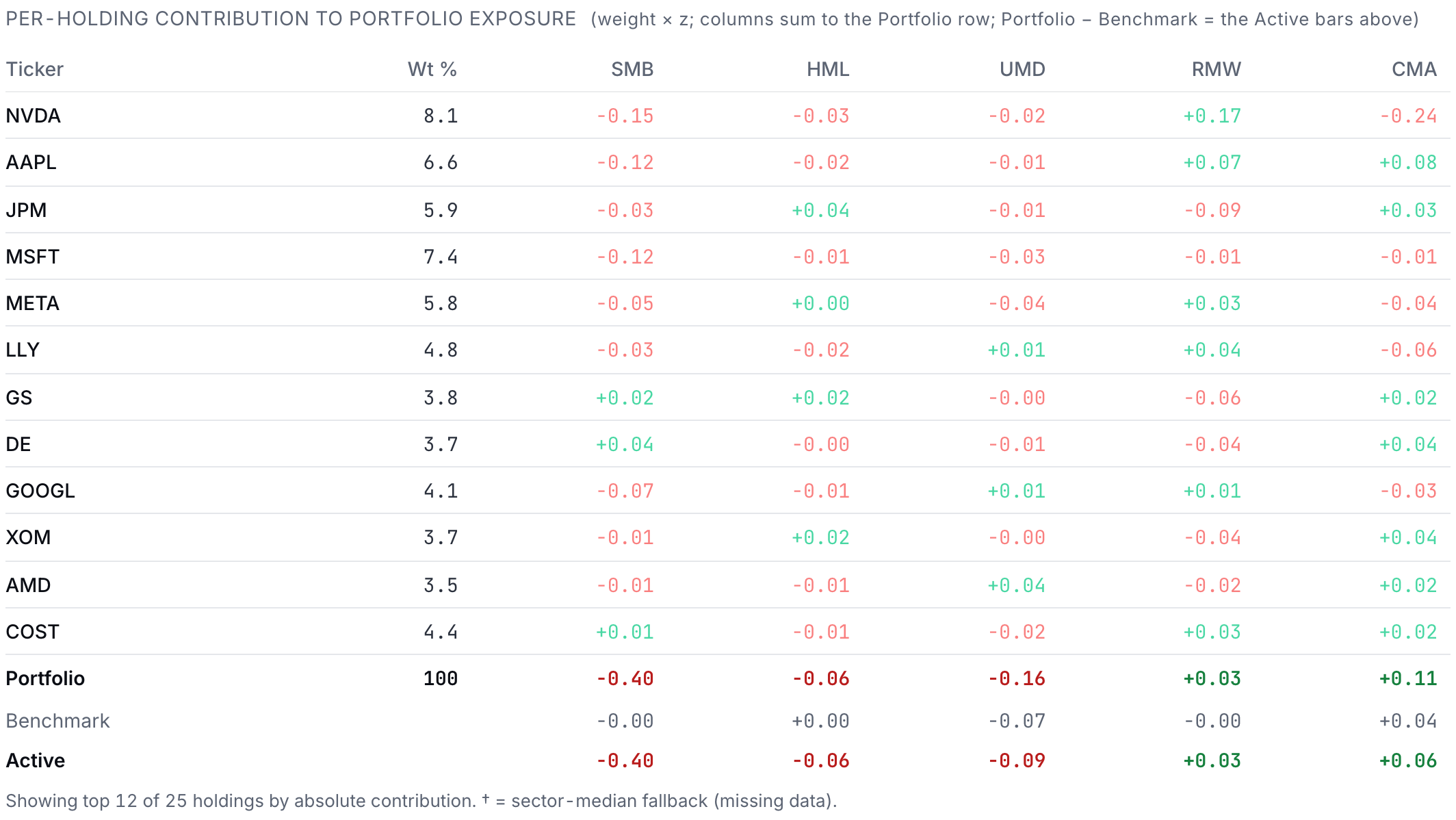
The card's lower half is that third step laid out for every holding, and the figure below shows it for the sample book. Each cell is weight × z, so the columns add up to the Portfolio row at the bottom, the Benchmark line under it shows the market's own score, and the Active line is the difference, which is what the bars above were drawing all along. A large cell tells you at once which position is carrying a tilt.
Practice
Momentum uses the trailing 12-month-minus-1 return. Universe mean +10%, std 8%. Your holding ran +30%. What is its Momentum z-score?
Solution. (30 − 10) / 8 = +2.5, which marks this holding as a strong recent winner. Notice the clip as well, because had the holding scored +3.4, the model would have recorded +3.0 instead (winsorization at work).
Lab: Lab: find your book's real bet
- Open Portfolio › Analyze › Diagnostics, choose Factor Tilts, and read the Factor Exposures card with the "Holdings-based" badge. (The Regression card below it, and the Risk Lab in Simulate, give return-based factor betas instead; those are a different measurement of the same idea.)
- Write down the two largest ACTIVE exposures (versus the benchmark), because that pair is your fund's actual style bet.
- Sanity-check one of them by hand. Pick your largest holding, estimate its characteristic (for example, is it bigger or smaller than the S&P average?), and confirm that the sign of its cell in the per-holding table matches. Each cell is weight × z with the weight as a fraction, so divide the cell by the weight to recover the z itself (a −0.15 cell on an 8.1% position is a z of about −1.85).
- Then go back to the correlation matrix and find your deepest red pair. If the two holdings share the sign of their largest factor cell, you have found the reason the matrix flagged them.
What it adds up to
Notice what we have done in this chapter. We started with a committee that counted its bets by sector label, built one cell of the correlation matrix by hand, and found that the count was wrong. We followed the correlation into the variance formula and saw that it, and not the number of holdings, decides how much diversification a book really has, and then we turned the factor panel on the same book in order to identify the bet that the matrix had only located. The pair chapter later in the book, Chapter 26, runs the same covariance term in reverse, because a long and a short that are highly correlated cancel most of their risk rather than doubling it. The matrix you can now read is the same one the fund's risk limits are written against, and Chapter 21 meets it there again, while Chapter 14 turns today's machinery around and asks what the weights would look like if the math chose them. Before any of that, one more chapter closes out this unit. The fund we have been analyzing as a single book is often run as several smaller ones, and Chapter 10 takes up the sleeves that carve it up and the three questions each sleeve gets asked.
Sources
- Markowitz, H. (1952). Portfolio selection. Journal of Finance, 7(1), 77-91 https://onlinelibrary.wiley.com/doi/10.1111/j.1540-6261.1952.tb01525.x
- Fama, E. F., and French, K. R. (1993). Common risk factors in the returns on stocks and bonds. Journal of Financial Economics, 33(1), 3-56 https://www.bauer.uh.edu/rsusmel/phd/Fama-French_JFE93.pdf
- Fama, E. F., and French, K. R. (2015). A five-factor asset pricing model. Journal of Financial Economics, 116(1), 1-22 https://www.sciencedirect.com/science/article/abs/pii/S0304405X14002323
- Jegadeesh, N., and Titman, S. (1993). Returns to buying winners and selling losers: Implications for stock market efficiency. Journal of Finance, 48(1), 65-91 https://www.bauer.uh.edu/rsusmel/phd/jegadeesh-titman93.pdf
The Analyst's Handbook is Sifter's textbook for student investors, written by Matt Lang and Bree Lang. Sifter is free for students. This chapter as markdown.