Chapter 3: Time-weighted return
The headline return, and why it ignores your deposits on purpose.
By Matt Lang and Bree Lang · About the authors
Where this is on Sifter: Portfolio · Analyze · Performance
Open Portfolio, then Analyze, and take a look at the large return figure at the top of the page. That number is a time-weighted return (TWR), and its job is to measure how good the investing was, regardless of when money happened to arrive or leave. Why would anybody want a return measure that ignores the timing of money? The best way to answer that question is with a problem that every student fund meets sooner or later.
Imagine that a generous alum wires your fund $50,000 in March. The fund is suddenly much bigger, but take a moment and ask yourself who earned that growth. Nobody on the investment team picked a stock, and the only skill on display belonged to the development office. So a return measure that leapt upward when the wire landed would be rewarding fundraising (a fine activity, but not the one we are trying to grade). In order to grade the investing by itself, we need a return that deposits and withdrawals (known in the trade as external flows) cannot move at all, and TWR is that return. In other words, the only thing that can change the TWR is what the holdings themselves did.
Sifter did not make this choice on its own. The industry's performance standard requires time-weighted returns for this very reason, which means that the number at the top of your Analyze tab is the same number a professional would ask for.1 The figure below shows the top of that tab on the sample book.
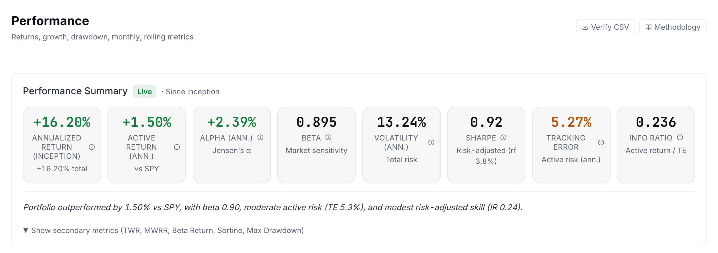
Before we go any further, take a minute and look at the row of tabs above the summary card, because the rest of this unit is on them. Performance, Dividends and Sleeves come first, and past a small Advanced mark come Attribution and Diagnostics, the two tabs that Chapter 8 and Chapter 7 will send you to. Further down the Performance tab you will also find three collapsed sections (Drawdown and beta, Monthly returns, and Rolling risk metrics) that open with a click on their headers. If you would rather one of them stayed open, the small Lock open pill on its header keeps it that way on every visit, which means that by the time Chapter 5 asks you to find the drawdown chart, it can already be waiting for you.
Daily return, flow-adjusted
is end-of-day portfolio value, is yesterday's end-of-day value, and is any external flow (deposit positive, withdrawal negative) that landed during day . The flow goes in the denominator: money that arrived today gets counted as capital you started with, so its arrival is not treated as a gain.
Chaining days together
Multiply each day's growth factor, then subtract 1. This is called geometric chaining. Returns compound, they do not add: two days of +1.00% is 1.01 × 1.01 − 1 = +2.01%, not +2.00%.
Check yourself
Your portfolio returns +10% one day and −10% the next. Where did you end up?
- Exactly where you started: +10% and −10% cancel. Unfortunately, they do not cancel, because 1.10 × 0.90 = 0.99. Adding returns instead of chaining them is the most common mistake people make when computing returns by hand.
- Down 1%. (correct) Right. 1.10 × 0.90 − 1 = −1.0%. Take a moment to think about why the two days do not cancel. The −10% was applied to a bigger base than the +10% was, so the down day took away more dollars than the up day added. This is why Sifter chains daily growth factors instead of adding percentages.
- Up 1%. Take another look at the order of operations. 1.10 × 0.90 = 0.99, which is a loss rather than a gain.
Now that we have both formulas, we need a dataset to practice them on, and we already have one. The Maple Fund, the small practice book whose ledger you replayed in Chapter 2, is the book we will work with for the rest of this unit. Its performance record covers ten trading days, and we have planted one event in the middle of it on purpose, because a stretch of plain days would not give the flow adjustment anything to do. On day 6, a donor wires in $1,000. The complete record, exact to the penny, is below.
Maple Fund: end-of-day values and flows
| Day | Date | External flow | End-of-day value |
|---|---|---|---|
| 0 | 2026-01-02 | baseline | $10,000.00 |
| 1 | 2026-01-05 | $10,100.00 | |
| 2 | 2026-01-06 | $10,049.50 | |
| 3 | 2026-01-07 | $10,069.60 | |
| 4 | 2026-01-08 | $10,069.60 | |
| 5 | 2026-01-09 | $10,145.12 | |
| 6 | 2026-01-12 | $1,000.00 | $11,256.57 |
| 7 | 2026-01-13 | $11,228.43 | |
| 8 | 2026-01-14 | $11,273.34 | |
| 9 | 2026-01-15 | $11,284.62 | |
| 10 | 2026-01-16 | $11,352.33 |
Day 0 is the starting point, so no return is measured for it. The values are exact to the cent. Carry four decimal places through your intermediate work and round only at the end.
Worked example: Worked example: the Maple Fund's 10-day TWR
Let's work through three of the daily returns by hand (the interesting ones), and then chain all ten together.
- Day 1: a plain day, no flow r₁ = V₁ / (V₀ + 0) − 1 = $10,100.00 / $10,000.00 − 1 r₁ = 1.00%
- Day 2: a down day r₂ = $10,049.50 / $10,100.00 − 1 r₂ = -0.50%
- Day 6: the $1,000 contribution arrives The flow goes in the denominator. r₆ = V₆ / (V₅ + F₆) − 1 = $11,256.57 / ($10,145.12 + $1,000.00) − 1 = $11,256.57 / $11,145.12 − 1 r₆ = 1.00%. The portfolio grew about $1,111.45 on the day, but $1,000.00 of that was the wire, not investing. The formula strips it out.
- Chain all ten days TWR = (1 + 0.0100) × (1 − 0.0050) × (1 + 0.0020) × (1 + 0.0000) × (1 + 0.0075) × (1 + 0.0100) × (1 − 0.0025) × (1 + 0.0040) × (1 + 0.0010) × (1 + 0.0060) − 1 TWR = 3.3373% over the ten days.
- Compare with the naive calculation Ending value over starting value: $11,352.33 / $10,000.00 − 1 = 13.52%. That number claims a 13.52% gain, but $1,000.00 of the increase was the donor's wire. Naive: 13.52%. True TWR: 3.34%. The difference is the entire reason this formula exists.
Practice
Your turn. Using the table above, compute the Maple Fund's day 8 return (from 2026-01-13 to 2026-01-14). Enter it as a percentage.
Solution. r₈ = $11,273.34 / $11,228.43 − 1 = 0.40%
Practice
Chain just the first three days (days 1, 2, 3) into a 3-day TWR. Enter it as a percentage to at least 2 decimal places.
Solution. (1.0100)(0.9950)(1.0020) − 1 = 0.6960%. If you had added the three percentages instead, you would have landed on 0.70%, which is close to the true answer here only because the daily returns are small. As the moves get bigger, the difference between adding and chaining grows quickly.
Practice
Here is a variant, in round numbers this time. A book closes at $10,000.00 on Tuesday. On Wednesday a $2,000.00 wire lands, and the book ends the day at $12,120.00. What is Wednesday's return, as a percentage?
Solution. $12,120.00 / ($10,000.00 + $2,000.00) − 1 = 1.00% exactly. Take a moment and compare this answer with the Maple Fund's real day 6, which was also 1.00% on a $1,000 wire. The manager's day is worth the same in both cases, because the flow never touches the return. This means that TWR is working as designed.
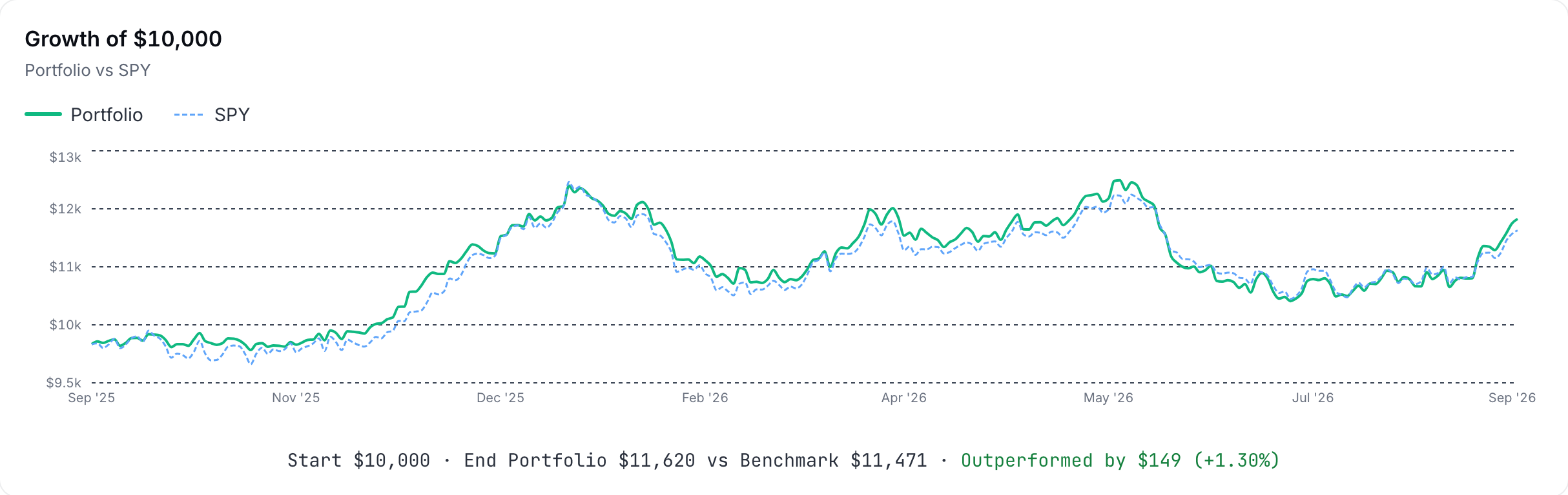
Every point on the Growth of $10,000 chart further down the Performance tab is this same chain, stopped at that day and applied to a notional $10,000, which is why a deposit never puts a step in the line. The figure below shows the chart on the sample book, and the Verify CSV button in the first figure hands you the daily series it was drawn from, which is what the lab that follows is built on.
Lab: CSV lab: reproduce the platform's return
- Go to Portfolio › Analyze › Performance and pick a period (1Y is fine, or Since inception if your book is younger than a year).
- Download the Verify CSV and open it in a spreadsheet. In its DAILY RETURNS section, the Portfolio Return column holds the daily rₜ values, already flow-adjusted, as decimals.
- In a new column compute (1 + rₜ) for each row, then multiply the whole column down with PRODUCT(). Subtract 1.
- Compare your result to the "Total Return" row of the same file's SUMMARY METRICS section. They should match to within rounding (a few hundredths of a percent).
There is one loose end to tie up before we move on. TWR ignores the timing of money on purpose, but the timing still mattered enormously to whoever chose it, and a complete picture of performance ought to have something to say about that choice. This is why the Performance tab shows a second return, the MWRR, tucked behind the same Show secondary metrics line as the TWR, whose entire job is to judge the thing that TWR refuses to. The two numbers disagree about the same portfolio all the time, and hopefully that strikes you as more interesting than alarming, because the next chapter will show that the disagreement is not a defect in either measure but a piece of information in its own right.
Sources
- CFA Institute (2019). Global Investment Performance Standards (GIPS) for Firms, 2020 edition. Effective 1 January 2020 https://www.gipsstandards.org/wp-content/uploads/2021/03/2020_gips_standards_firms.pdf
The Analyst's Handbook is Sifter's textbook for student investors, written by Matt Lang and Bree Lang. Sifter is free for students. This chapter as markdown.