Chapter 8: Attribution: which holdings earned the return

CTE, MCTE, and the Brinson split of allocation versus selection.

By Matt Lang and Bree Lang · About the authors

Where this is on Sifter: Portfolio · Analyze · Attribution

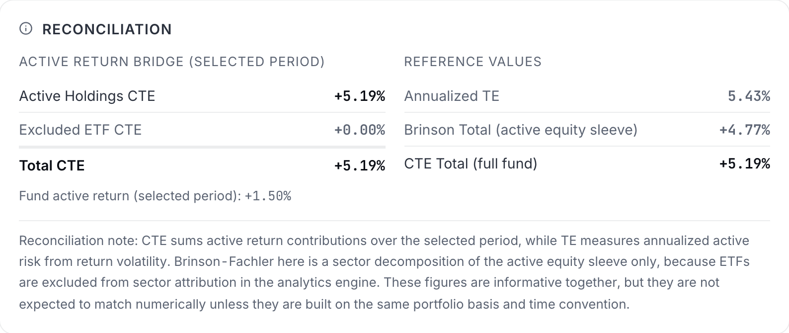
Imagine that you have just told an investment committee that your fund beat its benchmark this period. Take a moment and guess what the next question will be, because it is the same question in every committee room in the industry. The committee will want to know where the win came from, and "we are up" is not an answer (although it has certainly been tried). Attribution is the set of tools that turns "we are up" into an answer, and it splits the active return into named pieces in two different ways. The first split is by holding, which tells us which stocks did the work. The second split is by decision type, which asks whether we were better at picking sectors or at picking stocks within those sectors. That second split is the Brinson-Fachler decomposition, published in 1985 and still the arrangement that almost every performance report in the industry uses.¹ Because the two splits are carving up the same active return, they must add up to the same total, and the Attribution tab has a reconciliation card that puts the totals on screen rather than asking you to take them on faith. (On a real book, computed day by day over many periods, the two totals land close rather than identical, and the card also shows the fund's own active return, which includes the cash the equity sleeve does not hold.)

There is a lot of arithmetic ahead of us in this chapter, probably more than in any other chapter of the unit, but no single calculation in it is hard, and if you take the pieces one at a time they will fit together by the end. In order to keep the numbers manageable, we will work from a simplified period-level view of the Maple Fund, with three active stocks, one per sector, lined up next to their benchmark weights.

Maple Fund, sector view for the period

Sector (stock)	Port weight	Bench weight	Port return	Bench return
Technology (MPL)	60%	50%	5%	4%
Healthcare (BRC)	25%	30%	1%	1%
Energy (CDR)	15%	20%	-1%	0%
Total	100%	100%	3.10%	2.30%

Port is the Maple Fund's own weight in the sector and its return there; Bench is the benchmark's weight and return in the same sector. Multiplying each row's weight by its return and summing gives a portfolio return of 3.10% and a benchmark return of 2.30%, which means that the fund earned an active return of 0.80pp for the period. Every number in the rest of this chapter traces back to this table, so take a minute and make sure you feel good about it before moving on.

Contribution to excess return (CTE), per holding

$\text{CTE}_h \;\approx\; w_h \times \left( R_h - R_{b,\text{total}} \right)$

h is one holding, w_h is its weight in the fund, R_h is its return for the period, and R_b,total is the return of the ENTIRE benchmark, not of the holding's sector. How much of the active return this holding is responsible for: its weight times how far it beat (or trailed) the overall benchmark. The platform computes it from daily weights and returns; the single-period version here is the hand-calculable approximation. Index ETF positions are excluded from the per-stock list and shown as one "excluded ETF" line instead, since holding the benchmark is not an active decision.

Worked example: Worked example: CTE by holding

Let's take the three holdings one at a time, keeping in mind that the benchmark's total return for the period is 2.30%.

MPL (Technology) CTE = 60% × (5.00% − 2.30%) = 0.60 × 2.70pp +1.62pp. A big weight on a big winner, which drove the whole period.
BRC (Healthcare) CTE = 25% × (1.00% − 2.30%) = 0.25 × (−1.30pp) -0.33pp. It made money but less than the benchmark, so it DRAGGED the active return. Positive return, negative contribution: the distinction students miss most often.
CDR (Energy) CTE = 15% × (−1.00% − 2.30%) = 0.15 × (−3.30pp) -0.50pp.
Reconcile 1.62 − 0.33 − 0.50 = 0.80pp, exactly the fund's active return. The CTE column always sums to the total; if it does not, something is broken, which is why the tab shows a reconciliation card, pictured below on the sample book.

The reconciliation card on the Attribution tab of the sample book: an active return bridge with Active Holdings CTE, Excluded ETF CTE and Total CTE, the fund's active return for the selected period, and reference values for annualized tracking error, the Brinson total for the active equity sleeve and the full-fund CTE total. — **The reconciliation card, on the sample book.** The bridge sums the holdings' contributions to a Total CTE and compares it with the fund's active return. On this book the two are apart because the sample fund spent its first four months building positions and holding a great deal of cash, which the equity sleeve's contributions do not see. Pick a three-month window on the same page and the two figures land within a few hundredths of each other.

Brinson-Fachler: three effects per sector

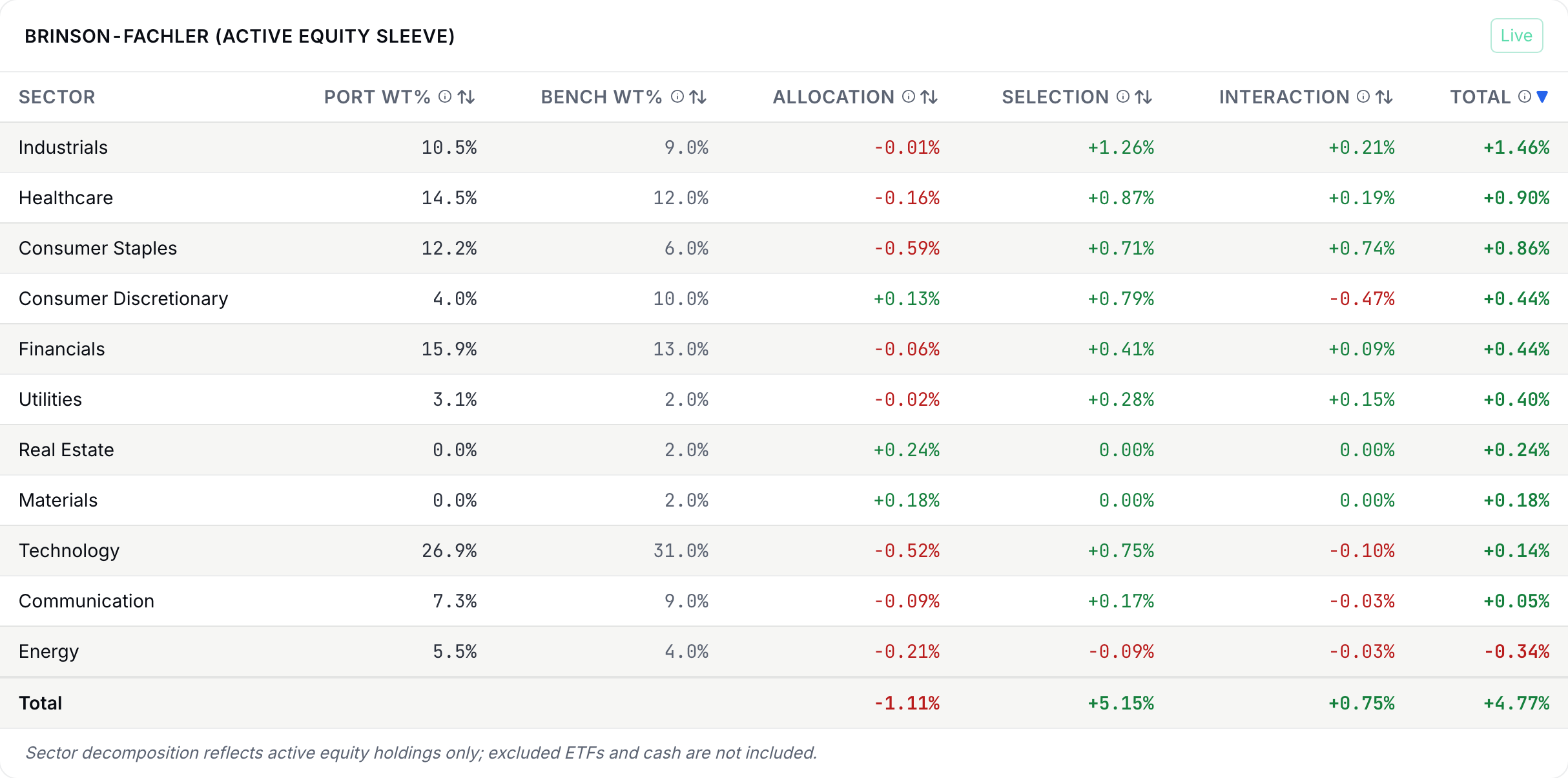
$\begin{aligned} \text{Alloc} &= (w_p - w_b)\left(R_{b,s} - R_{b,\text{tot}}\right) \\[2pt] \text{Sel} &= w_b \left(R_{p,s} - R_{b,s}\right) \\[2pt] \text{Inter} &= (w_p - w_b)\left(R_{p,s} - R_{b,s}\right) \end{aligned}$

For one sector s: w_p and w_b are the fund's and the benchmark's weights in it, R_p,s and R_b,s are the fund's and the benchmark's returns inside it, and R_b,tot is the whole benchmark's return (the Total row of the table above). Allocation: did you OVERWEIGHT sectors that beat the benchmark overall? Judged with benchmark sector returns only, so it isolates the sector-weighting decision. Selection: within each sector, did your stocks beat that sector's benchmark? Judged at benchmark weights. Interaction: the cross-term (overweighting a sector where you also picked well compounds both). The three effects sum to the sector's active contribution.

Worked example: Worked example: Brinson on the Technology sector

We will run all three effects on the Technology sector, where the portfolio put 60% into a stock that returned +5.00% while the benchmark gave the sector 50% and earned +4.00%, all against a benchmark total of 2.30%.

Allocation effect (60% − 50%) × (4.00% − 2.30%) = 0.10 × 1.70pp +0.17pp. You overweighted a sector that beat the market: credit for the sector call, even if your stock had only matched the sector.
Selection effect 50% × (5.00% − 4.00%) = 0.50 × 1.00pp +0.5pp. Your tech pick beat the tech benchmark: credit for the stock call, judged at the benchmark's weight.
Interaction (60% − 50%) × (5.00% − 4.00%) = 0.10 × 1.00pp +0.1pp. The bonus for doing both at once: extra weight on a stock that also outpicked.
Sector total, then fund total Technology contributes 0.77pp. Repeating for Healthcare (+0.065pp) and Energy (-0.035pp) and summing all effects across sectors: Allocation 0.35pp + Selection 0.30pp + Interaction 0.15pp = 0.80pp. Same total as the CTE column: two stories, one number. The Attribution tab runs this same split across every sector of your book, shown below on the sample book.

The Brinson-Fachler table on the Attribution tab of the sample book: one row per sector with portfolio weight, benchmark weight, allocation, selection, interaction and total columns, sorted by total. — **The Brinson-Fachler table, on the sample book.** One row per sector, the same three effects you just computed for Technology, judged against SPY's sector weights. Read any row with the formulas above: the allocation column is the weight difference times the sector benchmark's edge over the whole benchmark, and the selection column is the benchmark weight times your stocks' edge over the sector. Your sectors and numbers will differ.

Practice

Compute the Energy sector's allocation effect, in percentage points. (Portfolio weight 15%, benchmark weight 20%, Energy benchmark return 0.00%, benchmark total 2.30%.)

Solution. (15% − 20%) × (0.00% − 2.30%) = (−0.05) × (−2.30pp) = +0.115pp. Take a moment to think about why this comes out positive. You UNDERWEIGHTED a sector that went on to lag the market, which means that keeping money away from Energy was a good sector call, and the two negative factors multiply into a positive allocation effect.

Check yourself

A holding returned +4% over a period when the benchmark returned +7%. Its CTE is:

Positive: the stock made money. Remember that CTE measures the contribution to EXCESS return, not to return in general. A holding can make money and still trail the benchmark, and when it does, it is lowering the active return rather than raising it.
Negative: it trailed the benchmark, so it dragged on active return. (correct) CTE = weight × (4% − 7%) < 0. The difference inside the parentheses is what matters, and it is negative no matter how large or small the weight is. On the Attribution tab, this stock will be in the detractors column even though it went up, which means that a holding can be an absolute gain and a relative drag at the same time.
Zero: gains and benchmark-relative effects cancel. Nothing in the formula cancels. CTE is the weight times the difference in returns, and that difference here is −3pp, so the answer cannot be zero.

Marginal contribution to tracking error (MCTE), per holding

$\text{MCTE}_h \;=\; \frac{\text{Cov}(c_h,\, r_{\text{active}})}{\sigma(r_{\text{active}})} \times \sqrt{252}, \qquad c_h = w_h\, r_h$

c_h is the holding's daily contribution, its weight that day times its return that day, and r_active is the fund's daily active return (portfolio minus benchmark). Take the covariance of the two series over the window, divide by the standard deviation of the active returns, and annualize with √252. Because the active return is the sum of the contributions less the benchmark, these covariances add up to the variance of the active return, which is why the MCTEs sum to the tracking error; the platform rescales them slightly so the sum is exact even when a holding is missing a day of prices. A holding with a large MCTE moves WITH the fund's deviations from the benchmark; a negative one offsets them.

Everything in this chapter so far has taken the fund's holdings as given and asked which of them did the work. There is a second question that committees ask almost as often, and it tends to come up right after a big rebalance. Imagine that the fund sold ten positions on a Friday and bought thirteen new ones, and that two weeks later someone in the room asks, "would we have been better off if we had just left the book alone?" Attribution by holding cannot answer that, because it only looks at what the fund held and says nothing about what it gave up.

In order to answer it, we need a second book, one the fund never actually held. We start from the holdings as they stood at the close before the trades, let that book ride along with the market, and compare it day by day with the book the fund really owned. Because both books start from the same place and receive the same deposits and withdrawals, the difference between their returns comes from the trades and from nothing else. Performance reports often call this difference the trading effect (you will also see it called the timing effect), and it can go either way. In other words, a positive trading effect means the trades added to the return over the window, and a negative one means the fund would have done better by doing nothing at all.

Trading effect over a window

$\text{Trading effect} \;=\; R_{\text{actual}} - R_{\text{no-trade}}$

R_actual is the return of the book the fund held, and R_no-trade is the return of the same starting book with the trades taken out, both measured from the close before the first trade to the end of the window, with deposits and withdrawals left out of both. A trade the fund never made can be added to the second book the same way, which turns the question around to "what if we had bought it?"

Lab: CSV lab: verify one allocation effect

On Portfolio › Analyze › Attribution, download the Verify CSV, which comes in two sections (HOLDINGS ATTRIBUTION and SECTOR BRINSON-FACHLER).
In the Brinson section, pick whichever sector you like and pull its four inputs, which are Port Wt%, Bench Wt%, Bench Return% (the sector's benchmark return), and the benchmark total printed just above the table as "Benchmark total return used for Allocation". Use that line rather than the Performance file's Benchmark Total Return, because the sector split is computed on price returns from the window's first close to its last, while the Performance figure includes the benchmark's dividends, and the two can differ by a point or more over a year.
Compute (Port Wt − Bench Wt) × (Bench Return − benchmark total), divide by 100 to land in percentage points, and compare your answer with the Allocation% column. The inputs are printed to four decimals so the match should hold to the hundredth.
Lastly, sum the CTE column of the HOLDINGS ATTRIBUTION section and confirm it against the RECONCILIATION rows of the Diagnostics Verify CSV (Active Holdings CTE + Excluded ETFs CTE = Total CTE). That total is the equity sleeve's, so expect it to be near, not on, the fund's own active return whenever the book has held meaningful cash.

Sources

Brinson, G. P., and Fachler, N. (1985). Measuring non-US equity portfolio performance. Journal of Portfolio Management, 11(3), 73-76 https://jpm.pm-research.com/content/11/3/73

The Analyst's Handbook is Sifter's textbook for student investors, written by Matt Lang and Bree Lang. Sifter is free for students. This chapter as markdown.