Chapter 5: Volatility, Sharpe, Sortino, drawdown
Risk per unit of bumpiness, and the cost of only counting the bad bumps.
By Matt Lang and Bree Lang · About the authors
Where this is on Sifter: Portfolio · Analyze · Performance / Diagnostics
Imagine that two student funds are reporting their results for the year. The first fund, which we will call Granite, finished the year up 12% by way of a long and patient climb, and its worst week was barely noticeable. The second fund, which we will call Bottle Rocket, also finished up 12%, but its path ran through two steep collapses and three violent rallies. If you looked only at the bottom line, you would conclude that the two funds had the same year, but nobody who actually lived through both years would agree with you.
This means that the bottom line, all by itself, leaves out information that we badly want, and this chapter builds the four instruments that recover it (volatility, the Sharpe ratio, the Sortino ratio and drawdown). Fortunately, all four are built from material you already own, the daily return series from Chapter 3. The figure below draws both funds' years from their actual daily series, and every Granite and Bottle Rocket number in this chapter is computed from those same two series, so as each instrument arrives you can look back at the picture and see what it is measuring. By the end of the chapter you will be able to glance at a fund's statistics and tell a Granite from a Bottle Rocket, and that is the same skill a recruiter will be using when they read your fund's numbers.
Volatility (annualized)
Sample standard deviation (the n−1 version, STDEV.S in a spreadsheet) of the daily returns, scaled to a yearly number by the square root of 252 trading days. The √252 (not 252) is because independent randomness grows with the square root of time.
Practice
The Maple Fund's ten daily returns have a sample standard deviation of 0.5116% per day. Annualize it: what is the volatility, as a percentage? (Use √252 ≈ 15.8745.)
Solution. 0.5116% × 15.8745 = 8.12% annualized.
Volatility gives us a number for the wobble, and the numbers confirm what the figure above already showed, with Granite's year running at 9% annualized and Bottle Rocket's running at 24%. However, a big wobble on its own is not a verdict against a fund, because an investor might happily accept a rougher ride if the ride pays better, just as some travelers will fly a budget airline because the fare is low.
Before we can price the reward, we need a floor to measure it from, because part of any return required no risk at all. That floor is the risk-free rate (Rf), which is what the money would have earned parked in short-term U.S. government debt, known as Treasury bills (or "T-bills"), the standard stand-in for a return with no risk in it. This means that only the return above the floor, the excess return, is the part your risk actually paid for. What we need now is an exchange rate between risk and excess return, a number that tells us how much reward each unit of bumpiness bought. In 1966, an economist named William Sharpe supplied one, and his ratio has proven so durable that the industry simply named it after him.1
Sharpe ratio
Annualized return minus the risk-free rate, divided by annualized volatility: excess return per unit of total bumpiness. Sifter's risk-free rate is a Treasury yield matched to the window, the 3-month bill for windows under a year and the 1-year yield for longer ones, averaged across the years your period spans, and the Sharpe tile's subtitle on the Performance Summary shows the rate it used.
Worked example: Worked example: Granite versus Bottle Rocket
Both funds returned 12.0% for the year, and the risk-free rate was 5.3%. Granite ran at 9% volatility and Bottle Rocket ran at 24%. (The Sharpe ratio needs a long window of data to mean anything, and the callout below explains why.)
- The excess return, shared by both R_ann − Rf = 12.0% − 5.3% 6.7 percentage points over T-bills, for both funds. On the bottom line they remain identical twins.
- Granite Sharpe = 6.7% / 9.0% 0.74. Each unit of bumpiness bought Granite 0.74 units of excess return.
- Bottle Rocket Sharpe = 6.7% / 24.0% 0.28. The same reward, purchased with nearly three times the turbulence. The twins are twins no longer.
- Read the scale Rules of thumb on annual data: below 0 means T-bills won; 0.5 is respectable; 1.0 is strong; 2.0 or better on a long window should be treated with suspicion. Granite had a genuinely good year. Bottle Rocket had an adventure.
At this point the president of Bottle Rocket raises a fair objection. "Half my volatility was UPWARD. We had weeks where we made 6%. Why is the formula punishing good news?" This is the oldest complaint against the Sharpe ratio, and it is technically correct, because a standard deviation counts good surprises and bad surprises alike. Frank Sortino, who had spent years arguing that risk is what happens below the line you actually care about, eventually published the repair, a ratio that divides by the bad bumps only.2
Sortino ratio
Same numerator as Sharpe, but the denominator DD is the downside deviation (also called downside semideviation): it only counts returns below the daily risk-free target, and the Sortino-Forsey version divides by all n days, not just the down days3. Upside bumpiness stops being a sin.
Worked example: Worked example: downside deviation by hand
Imagine a fund having a Bottle Rocket sort of week, with five daily returns of +2%, −1%, +3%, −2% and +1%. The formula's target is the daily risk-free rate, but at 5.3% a year that works out to about 0.02% a day, so we will round the target to 0% and work in percent units throughout.
- Keep only the shortfalls min(0, r) day by day: min(0, +2) = 0, min(0, −1) = −1, min(0, +3) = 0, min(0, −2) = −2, min(0, +1) = 0 Two days fell short of the target. The three up days contribute exactly nothing, which is the whole idea.
- Square, average over ALL n days, square-root DD = √( (0 + (−1)² + 0 + (−2)² + 0) / 5 ) = √( (1 + 4) / 5 ) = √1 DD = 1.00% per day. Dividing by all 5 days (not just the 2 bad ones) is the Sortino-Forsey convention Sifter uses.3
- Now the full standard deviation, for contrast The mean return is (2 − 1 + 3 − 2 + 1) / 5 = 0.6%. Deviations from it: +1.4, −1.6, +2.4, −2.6, +0.4. Their squares sum to 17.2; divide by n − 1 = 4 (the STDEV.S convention from the volatility formula above) and take the root: √4.3 ≈ 2.07%. The full stdev is 2.07% per day, double the downside deviation, because the +2% and +3% rallies count toward it while contributing zero to DD.
- Compare the two Same five days, two risk numbers: 2.07% of total bumpiness, 1.00% of downside. A book whose bumps are mostly upward scores much better on Sortino than Sharpe. That asymmetry is the entire point of the metric.
Check yourself
Two funds both return 10% with 12% volatility, but Fund A's volatility is mostly up-moves and Fund B's is mostly down-moves. Which statement is right?
- Same Sharpe, same Sortino: the numbers cannot tell them apart. The Sharpe ratios are identical, but the Sortinos are not, because Sortino only penalizes the downside half of the movement.
- Same Sharpe; Fund A has the higher Sortino. (correct) Sharpe treats all variance alike, so the two funds tie on Sharpe. However, Sortino divides by the downside deviation only, which is small for Fund A and large for Fund B.
- Fund A has both a higher Sharpe and a higher Sortino. Sharpe uses total volatility, which is the same 12% for both funds, so it cannot separate them. Only the Sortino ratio can.
Volatility, Sharpe and Sortino are statistics that analysts read, but our last instrument measures something that investors physically live through. A client does not call the manager to complain that the annualized standard deviation has gotten large, but the phone rings quickly when a statement shows a third of the money gone. The number that records this experience is the drawdown, which is the fall from the highest point reached so far down to the lowest point that comes after it.
Drawdowns come with an unforgiving arithmetic that every analyst should internalize early. If you lose 10%, you need an 11% gain just to climb back to where you started, and if you lose 50%, you need a full 100% gain (a double!) to break even. Because of this, read the max drawdown literally. It describes the exact experience of the unluckiest person who ever invested with you, the one who arrived right at the peak and rode the fund all the way down to the trough.
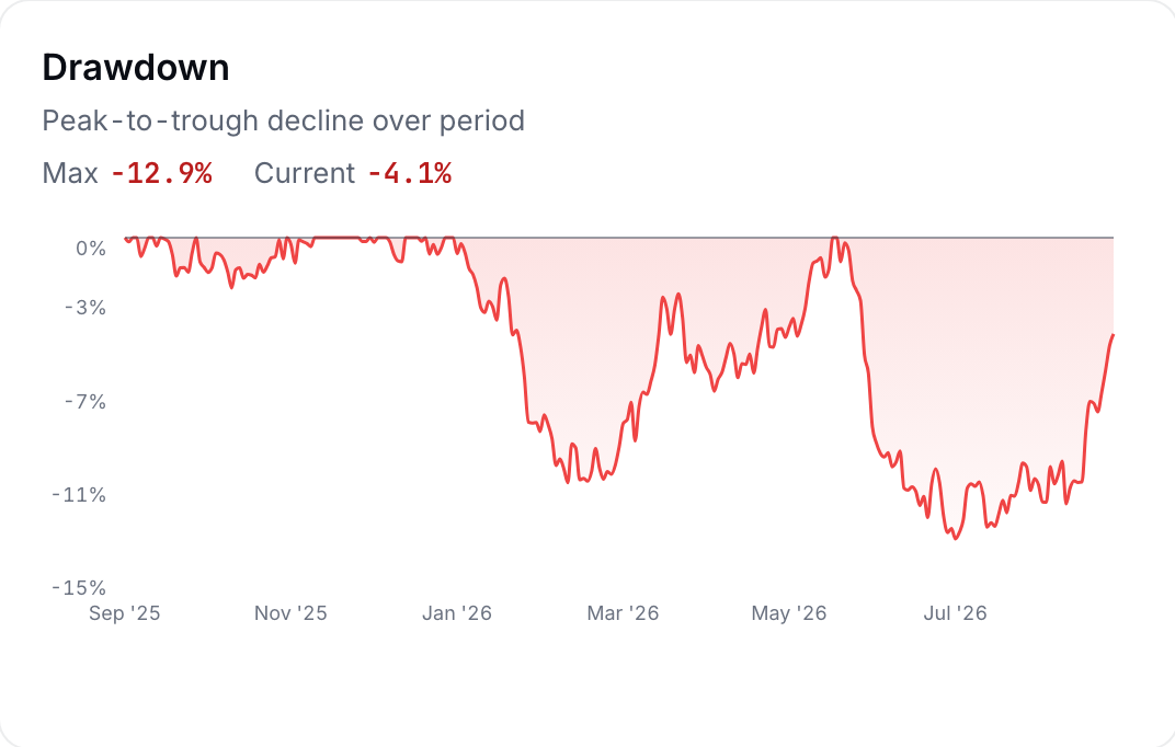
Run this walk on the two series from the opening figure and the last pair of numbers falls out. Granite's worst peak-to-trough fall for the year was 7%, a hole that a 8% rally refills. Bottle Rocket's second collapse carried it 30% below its high, a hole that takes a 43% climb to escape, and the violence of its rallies is the only reason it still finished the year up 12%. Its unluckiest investor, the one who bought at that high, watched 30 cents of every dollar disappear before the recovery began. Scroll back up to the figure and you can trace that exact experience on the red line. The Performance tab draws this same walk for your own book as its Drawdown card, shown below the formula on the sample book.
Maximum drawdown
Walk the cumulative growth path; at each day compare the current level to the highest level seen so far. The worst such drop is the max drawdown: the loss of the unluckiest possible entry-to-trough holder.
Practice
The Maple Fund's cumulative growth index over the ten days runs: 1.01000, 1.00495, 1.00696, 1.00696, 1.01451, 1.02466, 1.02210, 1.02618, 1.02721, 1.03337. What is the maximum drawdown, as a negative percentage?
Solution. Peak after day 1 = 1.01000; day 2 dips to 1.00495. (1.00495 − 1.01000)/1.01000 = -0.50% exactly. The later dip on day 7 (1.02210 against its 1.02466 peak) is only −0.25%, so day 2 is the max drawdown.
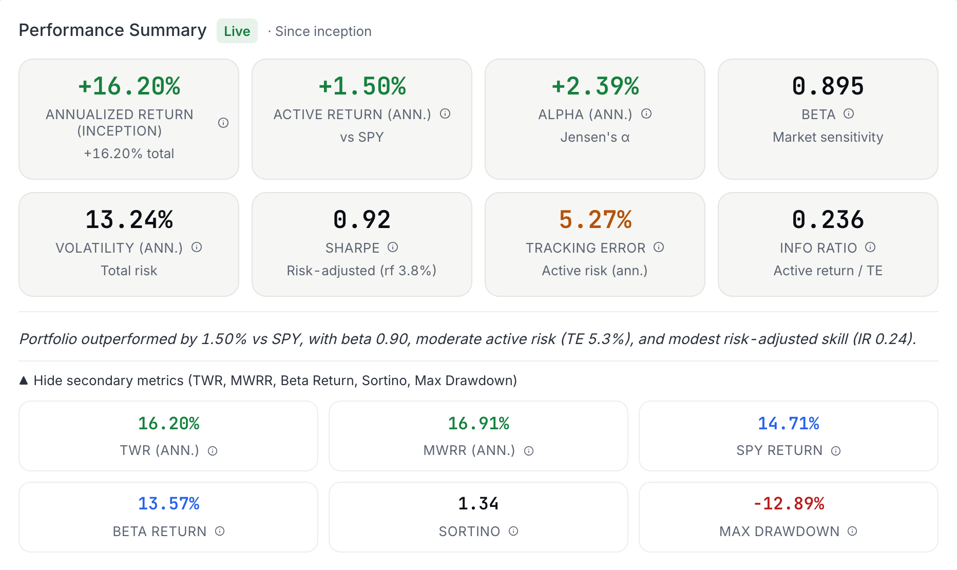
Let's return to our two funds and read their instruments side by side. Granite finished with a 12% return, 9% volatility, a Sharpe of 0.74 and a max drawdown of 7%. Bottle Rocket finished with the same 12% return, 24% volatility, a Sharpe of 0.28 and a max drawdown of 30%. Every one of those eight numbers is computed from the two daily series in the opening figure, and two funds that looked identical on the bottom line look nothing alike once the four instruments are read, and this is the information a reader of your fund's statistics is hoping to find. Before moving on, make sure you feel good about what each instrument measures, and then head to the lab below and compute one of them from the raw series yourself. On your own book, volatility and the Sharpe are on the top row of the Performance Summary card, and Sortino and max drawdown are on the secondary row that opens when you click Show secondary metrics. The figure below shows the card on the sample book with that row open.
Lab: CSV lab: volatility from the raw series
- On Portfolio › Analyze › Performance, download the Verify CSV, which has a SUMMARY METRICS section and a DAILY RETURNS section.
- In a spreadsheet, run STDEV.S over the DAILY RETURNS section's Portfolio Return column.
- Multiply by SQRT(252). Compare with the "Volatility (Ann.)" row of the SUMMARY METRICS section.
- Bonus: build the cumulative growth column with a running product of (1 + r), track the running MAX, and reproduce Max Drawdown too.
Sources
- Sharpe, W. F. (1966). Mutual fund performance. Journal of Business, 39(1), Part 2, 119-138 https://finance.martinsewell.com/fund-performance/Sharpe1966.pdf
- Sortino, F. A., and van der Meer, R. (1991). Downside risk: Capturing what's at stake in investment situations. Journal of Portfolio Management, 17(4), 27-31 https://jpm.pm-research.com/content/17/4/27
- Sortino, F. A., and Forsey, H. J. (1996). On the use and misuse of downside risk. Journal of Portfolio Management, 22(2), 35-42 https://jpm.pm-research.com/content/22/2/35
The Analyst's Handbook is Sifter's textbook for student investors, written by Matt Lang and Bree Lang. Sifter is free for students. This chapter as markdown.