Chapter 6: Beta, alpha, and active return
How much of your return was the market, and how much was actually you.
By Matt Lang and Bree Lang · About the authors
Where this is on Sifter: Portfolio · Analyze · Performance / Diagnostics
Suppose your fund made 15% in a year when anyone patient enough to hold an index fund made 20%. Was that a good year? Take a moment and try to defend an answer in either direction, because the question is harder than it looks. Every return is really two things tangled together, the part the market handed you and the part your decisions added or subtracted, and no verdict is possible until the two are untangled. Untangling them is the work of this chapter, and it takes three numbers of increasing subtlety, active return, beta and alpha. Two of the three come with Greek letters attached, but the ideas behind the Greek letters are no harder than the arithmetic behind the plain ones. There is also a score to settle, because Chapter 5 left an argument hanging, and Granite and Bottle Rocket are returning for a second act.
Active return
R_p is the portfolio's return for the period and R_b is the benchmark's, both time-weighted and dividend-adjusted, so the difference comes out in percentage points. The benchmark is whichever one is selected on the Analyze toolbar (SPY by default). Active return is the simplest scorecard there is, and its weakness is that it says nothing about how much risk you took to earn it, which is the question that beta and alpha below exist to answer.
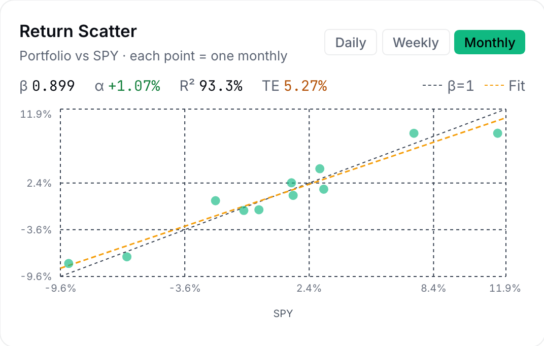
Let's start with a pattern you can observe for yourself during your first week of watching any portfolio. On most days, most stocks move together, and the thing they are all moving with is the market. Some portfolios feel every market swing at full strength, some feel a muffled version, and a few barely feel the market at all. Beta is the number that captures the difference, because it measures how hard your portfolio moves when the market moves. A beta of 1 means you rise and fall with the market one for one, which is what index funds do on purpose. Bottle Rocket has a beta of 1.6, which means that every market move reaches it amplified by sixty percent, in both directions. Granite's 0.6 means the same moves arrive dampened. A beta near zero means the market barely touches you (cash behaves this way), and a negative beta, which is rare, belongs to assets that tend to rise when everything else is falling. Beta is a slope, and the Performance tab draws that slope for your own book as its Return Scatter card, shown below the formula on the sample book.
Beta
Computed on daily returns. Beta is the slope of your returns against the market's: β = 1.2 means a day the benchmark moves +1%, you tend to move +1.2%. It needs at least 30 daily observations or Sifter shows nothing rather than noise.
Before the next formula, take a moment and ask yourself why the return you should expect from a portfolio would scale with beta, and with nothing else. The answer is one of the few genuinely deep ideas in finance, and it earned William Sharpe a share of a Nobel Prize.1 Think about the risks that belong to one company alone, such as your retailer fumbling a holiday season or your biotech's molecule failing. Risks of that kind can be diversified away almost for free, because when you hold thirty stocks, the individual stumbles largely cancel each other out. (Thirty is not a folk number. The study that fixed it in the textbooks put the floor at about thirty for a borrowing investor and forty for a lending one, at a time when the common belief was that ten would do.)5 Because anyone can shed company-specific risk this cheaply, the market refuses to pay anyone for carrying it. The only risk that cannot be diversified away is exposure to the market itself, and so, in the capital asset pricing model (CAPM), the only risk with a built-in reward is beta. This means that the bracket in the formula below can be read in plain words. It is the risk-free rate, plus your share of the market's payment for carrying market risk, and it is what a portfolio with your beta would have earned with no skill involved at all. Whatever you earn beyond the bracket was not owed to you, and it had to be taken, by judgment or by luck. That leftover goes by the most coveted letter in the business.
Alpha (Jensen's)
R_p is the portfolio's return over the window, R_b is the benchmark's (the market's, when the benchmark is SPY), Rf is the risk-free return over the same window, and β is the beta we just computed. The bracket is the prediction of the capital asset pricing model (CAPM): what a no-skill portfolio with your beta should have returned. Alpha is what you earned beyond that prediction. It is the risk-adjusted version of active return: a high-beta fund in an up market gets credit only for beating its handicap. The measure is Michael Jensen's, from a 1968 study that applied it to 115 mutual funds and found very little of it.2
Now let's bring Granite and Bottle Rocket back for their second act. Say the market returned 10.0% in their year, with the risk-free rate at our usual 5.3%. Both funds returned 12.0%, which means that both earned an active return of +2.0 points, and on that blunt measure they are still twins. The two funds took very different roads to the same 12.0%, however. Granite ran the year at a beta of 0.6, gliding along at six-tenths of the market's swing, while Bottle Rocket ran at 1.6, and that arrangement is what produced their 9% and 24% volatilities in the first place. Feed each fund through the CAPM bracket, and the scoreboard below changes completely.
Same return, opposite verdicts
| Fund | Return | Active | Beta | CAPM expected | Alpha |
|---|---|---|---|---|---|
| Granite | 12.0% | +2.0pp | 0.6 | 8.12% | +3.88pp |
| Bottle Rocket | 12.0% | +2.0pp | 1.6 | 12.82% | −0.82pp |
CAPM expected = 5.3% + beta x (10.0% − 5.3%). Take a moment with the last column, because Bottle Rocket beat the market and still earned a NEGATIVE alpha. With that much market exposure, in a market this good, a no-skill fund was supposed to win by more than Bottle Rocket did. Granite, meanwhile, beat its modest handicap by nearly four points, and the argument that active return left in a tie is settled in the quiet fund's favor.
Worked example: Worked example: Maple Fund beta and alpha
Let's compute beta first (a covariance is just an average of products of deviations), and then take alpha from the CAPM bracket.
- Mean daily returns Portfolio mean = 0.3300% per day; benchmark mean = 0.2500% per day. Deviations are measured from these means.
- Covariance: average the products of deviations For each day, multiply (portfolio deviation) × (benchmark deviation); sum the ten products; divide by n − 1 = 9. Day 1, for instance: (1.00% − 0.33%) × (0.80% − 0.25%) ≈ +0.369 %². Cov = 0.1878 (in %² units, that is 1.878e-5 in decimals).
- Variance of the benchmark, same recipe Square each benchmark deviation, sum, divide by 9. Var = 0.1494 %², so β = 0.1878 / 0.1494 = 1.26.
- Read the beta β = 1.26: the Maple Fund swings about 26% harder than its benchmark, both directions. An aggressive little fund.
- CAPM's prediction for that beta Over the 10 days the risk-free return is 0.2051% (5.3% annual, scaled to the window). Prediction = 0.2051% + 1.26 × (2.5214% − 0.2051%) Prediction = 3.1156%.
- Alpha is the leftover α = 3.3373% − 3.1156% α = 0.22pp over the period. Less than the raw active return of 0.82pp, because a 1.26-beta fund in an up market was supposed to win by some margin.
Check yourself
A fund with β = 1.5 returns 18% while the benchmark returns 14% (risk-free 4%). Its active return is +4pp. Its alpha is:
- Also +4pp: alpha and active return are the same thing. Alpha and active return only agree when beta equals 1, and this fund has a beta of 1.5. CAPM expected this fund to earn 4% + 1.5 × 10% = 19%.
- Negative: it underperformed its risk. (correct) The CAPM prediction is 4% + 1.5 × (14% − 4%) = 19%, and the fund made 18%, which means that α = −1pp. The fund beat the benchmark and still lost to its own handicap, which is the Bottle Rocket story all over again.
- Positive but smaller than +4pp. The reasoning is close, but the sign comes out wrong. Run the CAPM bracket and you get 4% + 1.5 × 10% = 19% expected, versus 18% earned, so the fund fell short of its handicap rather than clearing it by a little.
Practice
Your book has β = 0.8. The benchmark returns 10% and the risk-free rate is 5%. What return does CAPM predict for a no-skill portfolio with your beta, as a percentage?
Solution. 5% + 0.8 × 5% = 9.0%. This means that anything you earn above 9% is alpha, and earning "only" 9.5% in this market is genuine skill, even if it is a modest amount of it.
No number in finance carries more cultural weight than alpha. Funds name themselves after it, newsletters chase it, and a sizable share of the industry's fee structure rests on the claim of producing it. Against all of that, William Sharpe wrote down an argument that every analyst should be able to repeat from memory.3 The market is nothing other than the sum of everyone holding it, which means that in aggregate, before costs, the average actively managed dollar must earn exactly the market return, and after costs the average active dollar must therefore earn less. In other words, alpha is a zero-sum game played for an entry fee. (The argument does have one serious modern challenge, and you should know it if you ever have to defend active management. Sharpe's identity assumes a market portfolio that never changes, and real indices change all the time, because shares are issued and repurchased and indices are reconstituted. Allow for that and active managers can be worth positive fees in aggregate.)4 So where does all of this leave a student fund? A risk-adjusted alpha against the right benchmark, one a reader can check, is a claim most professionals cannot truthfully make, expressed in a number most students never learn to compute, and you have now worked through every step of computing it. The lab below asks you to do it once more in a spreadsheet, where the whole calculation collapses into a single function.
Lab: CSV lab: beta with SLOPE()
- On Portfolio › Analyze › Performance, download the Verify CSV. The DAILY RETURNS section has the columns you need, and the SUMMARY METRICS section has the reference values.
- In a spreadsheet: =SLOPE(portfolio_return_column, benchmark_return_column). SLOPE computes Cov/Var in one call, which is exactly the beta formula.
- Compare with the "Beta" row of the SUMMARY METRICS section.
- Bonus: =COVARIANCE.S(p, b) / VAR.S(b) gives the identical number the long way.
Sources
- Sharpe, W. F. (1964). Capital asset prices: A theory of market equilibrium under conditions of risk. Journal of Finance, 19(3), 425-442 https://onlinelibrary.wiley.com/doi/10.1111/j.1540-6261.1964.tb02865.x
- Jensen, M. C. (1968). The performance of mutual funds in the period 1945-1964. Journal of Finance, 23(2), 389-416 https://onlinelibrary.wiley.com/doi/10.1111/j.1540-6261.1968.tb00815.x
- Sharpe, W. F. (1991). The arithmetic of active management. Financial Analysts Journal, 47(1), 7-9 https://www.tandfonline.com/doi/abs/10.2469/faj.v47.n1.7
- Pedersen, L. H. (2018). Sharpening the arithmetic of active management. Financial Analysts Journal, 74(1), 21-36 https://www.tandfonline.com/doi/full/10.2469/faj.v74.n1.4
- Statman, M. (1987). How many stocks make a diversified portfolio?. Journal of Financial and Quantitative Analysis, 22(3), 353-363 https://www.cambridge.org/core/journals/journal-of-financial-and-quantitative-analysis/article/abs/how-many-stocks-make-a-diversified-portfolio/CE5CDF2C7225FC1E0EDE3E700A3C66A7
The Analyst's Handbook is Sifter's textbook for student investors, written by Matt Lang and Bree Lang. Sifter is free for students. This chapter as markdown.