Chapter 13: Stress tests, VaR, and CVaR

What a bad day costs, three ways of estimating it, and the fine print.

By Matt Lang and Bree Lang · About the authors

Where this is on Sifter: Portfolio · Simulate · Stress Test / Risk Lab

Chapter 5 measured how bumpy the ride has been, and measuring backward is the easy direction, because the past does not change while we measure it. A risk committee does not have that luxury. The question a committee brings into the room faces forward, and it usually arrives in blunt form, how much can we lose, and how often? Sifter comes at the question from two directions, with the scenario stress test asking, "what would 2008 do to this exact book?", and Value at Risk (VaR) asking, "what does an ordinarily bad day cost?" You may be tempted to crown one of these the better tool, but they are complements rather than rivals. VaR describes the routine tail, while stress tests describe days that are so far outside the routine that VaR, because of the way it is constructed, cannot imagine them. In other words, VaR prices the ordinary bad day, and a stress test replays an extraordinary one against the exact portfolio you hold today. Let's start with the stress test, since its arithmetic is the friendlier of the two.

Stress test: pushing a scenario through the book

r_h = \beta_h \, R_{\text{mkt}} + \left( R_{\text{sector}} - R_{\text{mkt}} \right),r_{\text{port}} = \sum_h w_h \, r_h

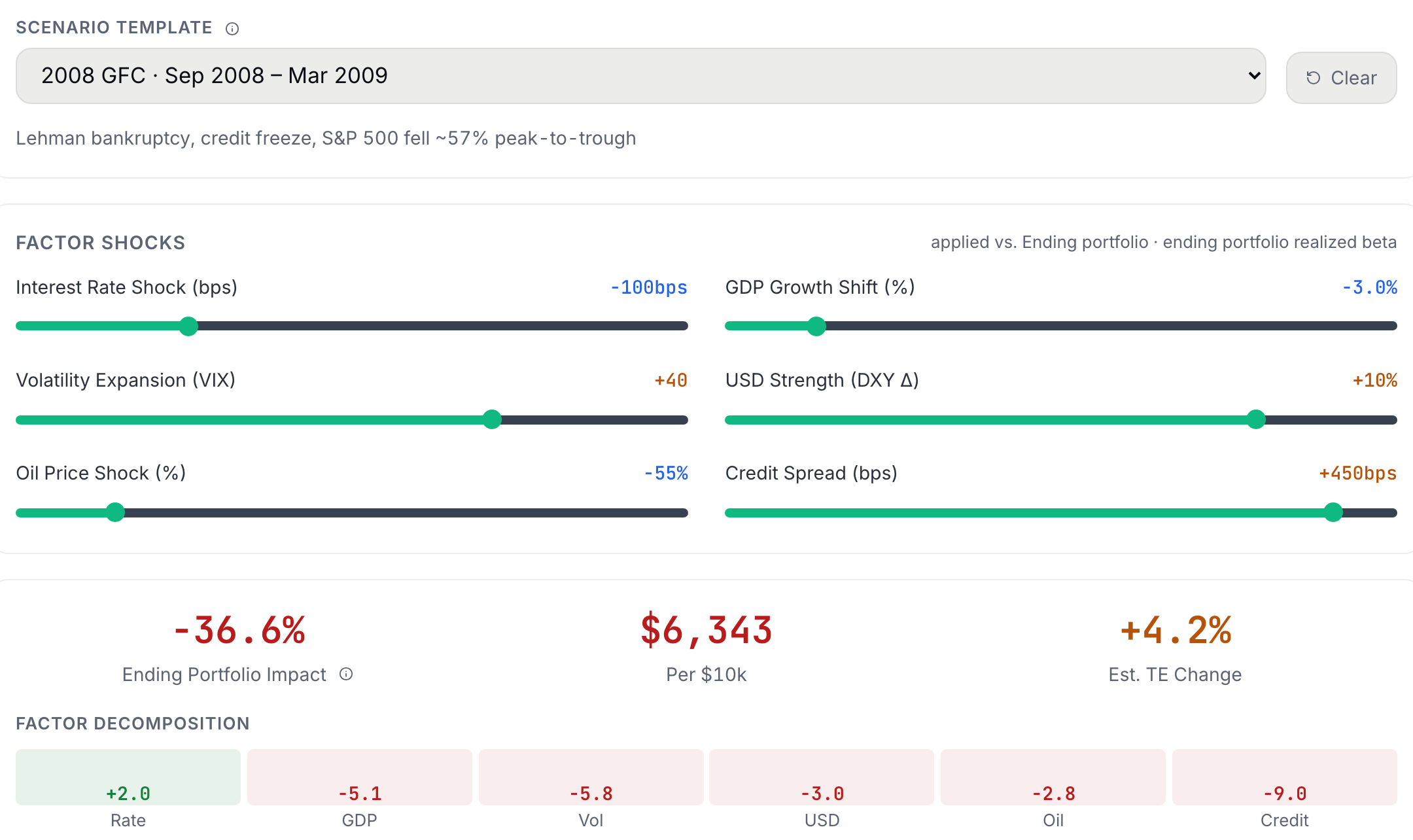
A scenario is a market shock plus sector offsets (the 2008 scenario hits Financials far harder than the market). In the first line, r_h is holding h's stressed return, β_h is its beta (Chapter 6), R_mkt is the scenario's market shock and R_sector is the shock to the holding's sector, so the holding inherits the market move through its beta and then takes its sector's extra kick on top. In the second line, w_h is the holding's weight and the portfolio's stressed return is the weighted sum. The Stress Test mode's six sliders come in two groups. Interest rates, GDP growth and VIX set the market shock, which reaches each holding through its beta. The dollar, oil and credit spreads do not go through beta at all, and they do not care what you hold, because each one adds the same amount to every holding's return, so a move in oil shifts your utility and your oil driller by the same number of points. That is a simplification, and it is the reason the sector offsets exist. Each holding's stressed return is capped at −95% and +250%, and a holding whose sector the scenario does not name is left at zero and flagged rather than guessed.

Practice

A scenario sets the market at −20% and the Energy sector at −30%. Your energy holding has β = 1.1 and a 15% weight. How many percentage points does this single holding contribute to the portfolio's stressed return?

Solution. r = 1.1 × (−20) + (−10) = −32%. Contribution = 15% × (−32%) = −4.8pp. Notice that the sector offset (−10) stacks on top of the beta-scaled market move, which means the holding takes the market's fall through its beta and then the sector's extra fall on top of that.

On the platform the scenario arrives as a template. Pick one and the six factor sliders jump to the values that episode actually printed, the sector offsets load behind them, and the headline impact appears beneath, as the figure below shows for the sample book with the 2008 template loaded. You can also start from zero and drag the sliders yourself, which is the right way to answer a committee member who asks what a particular rate shock would do.

The Stress Test mode on the sample book with the 2008 GFC template selected: a scenario picker with a one-line description, six factor sliders set to the template's values for interest rates, GDP growth, VIX, the dollar, oil and credit spreads, then the ending portfolio impact as a percentage and per $10,000, an estimated tracking-error change, and a factor decomposition row. — **The 2008 template, on the sample book.** The sliders are the scenario's inputs and the headline is the weighted sum of every holding's stressed return, capped as the formula above describes. The factor decomposition splits the part of the shock the sliders explain, which is why its cells do not add up to the headline on their own; the rest rides in through each holding's beta and sector. Your numbers will differ.

Value at Risk came out of one bank. In the early 1990s, Dennis Weatherstone, the chairman of J.P. Morgan, grew tired of thick risk reports that did not agree with one another, so he demanded something simpler. He wanted a single page on his desk at 4:15 each afternoon, fifteen minutes after the close, stating how much the bank could plausibly lose the next day. Take a moment to think about what that request forced the firm to do. In order to produce the "4:15 report", every position in every currency had to be compressed into one number, and the methodology built for the compressing was later given away to the world under the name RiskMetrics.⁴ That one number has been indispensable ever since, and it has been mildly dangerous for just as long, because a single number gets more confidence than it deserves. Fortunately, computing it requires nothing more than a pocket calculator, and we will do the computing right now.

Parametric VaR (the normal-curve estimate)

$\text{VaR}_{\alpha} \;=\; \mu_d - z_{\alpha}\, \sigma_d \qquad \left( z_{95} = 1.645, \;\; z_{99} = 2.326 \right)$

Here μ_d is the average daily return over the window and σ_d is the standard deviation of those daily returns (the volatility of Chapter 5, before it is annualized). The z value says how many standard deviations below the mean the cutoff is, and it comes straight from the normal curve, where a line 1.645 standard deviations below the mean leaves 5% of the days beneath it and a line 2.326 below leaves 1%. This means that if daily returns were normal, the 95% VaR is the loss exceeded only on the worst 5% of days. Sifter reports 1-, 5- and 10-day horizons at 95% and 99% (a multi-day figure scales the drift by the number of days and the volatility by the square root of the number of days). The Risk Lab shows the parametric figure next to two competitors precisely because the normality assumption is the weak link.

Worked example: Worked example: 1-day 95% VaR for the Maple Fund

Let's run the Maple Fund through the formula. Its daily mean is 0.3300% and its daily standard deviation is 0.5116%.

Plug into the formula VaR_95 = 0.3300% − 1.645 × 0.5116% = -0.51%. Read: on 19 days out of 20, the Maple Fund should do better than a 0.51% loss.
In dollars On the ending net asset value (NAV) of $11352, that is 0.51% × 11352 ≈ $58 on a normal-bad day.
What VaR does NOT say Nothing about the 20th day. VaR is a threshold, not a worst case: it tells you where the tail starts, not how deep it goes. The "how deep" question belongs to CVaR.

Practice

The demonstration above draws the 95% and 99% lines. Draw the 90% line yourself. Compute the Maple Fund's 1-day 90% parametric VaR, with z = 1.282, as a negative percentage.

Solution. 0.3300% − 1.282 × 0.5116% = -0.33%. Line the three thresholds up and take a moment to watch them march. Loosening the confidence to 90% pulled the line in to -0.33%, the worked example's 95% put it at -0.51%, and tightening to 99% pushes it out to -0.86%, which means that the same ten days of history can be made to say that a routine bad day costs a third of a point or most of a full point, depending on which tail you ask about. The deep tail is where the normal assumption is at its weakest.

CVaR, the average of the bad tail

VaR tells us where the tail begins and nothing more, so we need a companion measure for how bad the tail actually is. Conditional VaR (also called expected shortfall) answers the question, "GIVEN a worse-than-VaR day, how bad is it on average?" Instead of pointing at the threshold, it averages every loss beyond the threshold. This distinction matters more than it may first appear, because two books can share the same VaR while one of them hides a far nastier tail, and CVaR is the number that tells those two books apart. The bank regulators came around to the same view, and the Basel market-risk framework now requires banks to compute expected shortfall daily for the internal models that set market-risk capital, in place of the value at risk that the last crisis showed underestimating the days that mattered.³ Risk theory prefers CVaR as well, because unlike VaR it behaves properly when portfolios are combined, and the risk of the whole is never more than the sum of the parts.¹

The parametric figure trusts the normal curve to describe your tail, and the Risk Lab shows two other ways of drawing the same line. Historical VaR trusts nothing but the record. Sort the window's actual daily returns from worst to best and read off the 5th percentile, the return that only one day in twenty falls below (the platform, like a spreadsheet's PERCENTILE.INC, interpolates between the two nearest days when the percentile lands between them). No curve is assumed, but the method can never report a day worse than the worst day the window happened to contain, and a short calm window will hand you a comforting number for that reason alone. Cornish-Fisher VaR falls between the two. It starts from the normal z value and bends it by the skew and excess kurtosis measured in the record, so a history with a fat left tail gets a deeper line than the plain normal curve would draw. When the three disagree, you should report the disagreement, and the quiz below is about the most common way they disagree.

Check yourself

The Risk Lab shows VaR three ways: parametric, historical (the empirical tail of your actual days), and Cornish-Fisher (adjusted for skew and fat tails)². Your book's history is 60 days with no day worse than −1.2%. The historical 99% VaR comes out at −1.2%. What is the caveat?

Historical VaR is the most accurate of the three; trust it. With only 60 observations to work from, the empirical tail is nearly empty, and the methodology states the limit plainly. The historical method can never report a day worse than the worst day you happened to live through.
A short window's historical VaR cannot be worse than its worst observed day, so it understates the true tail. (correct) Right. A run of sixty calm days hands you a falsely comforting −1.2%, and this is the reason the three methods appear side by side in the Risk Lab. When they disagree, the disagreement itself is what you should be reporting.
Cornish-Fisher should always be ignored on small samples. This has it backwards. The skew and kurtosis adjustment in Cornish-Fisher is one way of estimating a tail depth that the short historical window has no way of showing you.

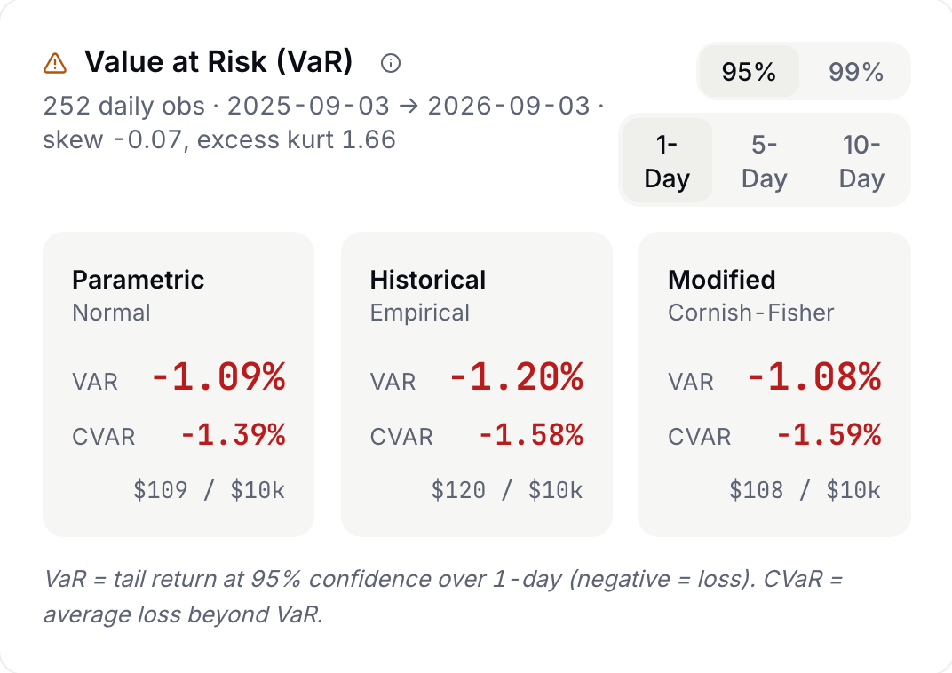
The figure below shows the Risk Lab's card for the sample book. The header states the window and the observation count, along with the skew and excess kurtosis of the daily series, which are the two numbers Cornish-Fisher uses to bend the normal quantile. Then the three methods sit side by side at the same confidence and horizon. On this book the historical figure is the deepest of the three, which is the fat left tail showing itself in the empirical percentile, and that is exactly the kind of disagreement the lab asks you to look for.

The Risk Lab Value at Risk card on the sample book: a header with the observation count, date range, skew and excess kurtosis, toggles for 95% and 99% confidence and 1-, 5- and 10-day horizons, and three columns for Parametric Normal, Historical Empirical and Modified Cornish-Fisher, each with a VaR and a CVaR figure and the dollar loss per $10,000. — **Value at Risk three ways, on the sample book.** One day, 95% confidence, three methods. VaR is the threshold and CVaR is the average loss beyond it, so within each column the second number is always the deeper one. Read across and the three thresholds disagree by about a tenth of a point, which on a calm year is a small argument; on a book with a nastier history the columns spread apart, and the spread is the finding.

Lab: CSV lab: historical VaR from the raw series

On Portfolio › Analyze › Performance, download the Verify CSV and use its DAILY RETURNS section.
In a spreadsheet, run PERCENTILE.INC(portfolio_return_column, 0.05). That is your empirical 1-day 95% VaR.
Compare with the Risk Lab's historical VaR at 95%, 1-day, after loading your current portfolio in Simulate over the same window. Expect the two to be close but not identical, because the Risk Lab runs on the synthetic book from Chapter 11 (constant weights, no dividends) while the CSV is your real daily record; a difference of more than a couple of tenths says your actual trading or your cash changed the tail.
Then compare with the parametric figure: μ − 1.645σ using AVERAGE and STDEV.S of the same column. If parametric is milder than historical, your return distribution has a heavier left tail than the normal curve assumes.

Sources

Rockafellar, R. T., and Uryasev, S. (2000). Optimization of conditional value-at-risk. Journal of Risk, 2(3), 21-41 https://www.semanticscholar.org/paper/Optimization-of-conditional-value-at-risk-Rockafellar-Uryasev/58444c142b6ea5c71a435cac7a0b4c66d6c68869
Fisher, R. A., and Cornish, E. A. (1960). The percentile points of distributions having known cumulants. Technometrics, 2(2), 209-225 https://www.stat.cmu.edu/technometrics/59-69/VOL-02-02/v0202209.pdf
Basel Committee on Banking Supervision (2019). Minimum capital requirements for market risk. Bank for International Settlements (the Fundamental Review of the Trading Book) https://www.bis.org/bcbs/publ/d457.pdf
J.P. Morgan and Reuters (1996). RiskMetrics technical document (4th edition). First published October 1994 https://www.msci.com/documents/10199/5915b101-4206-4ba0-aee2-3449d5c7e95a

The Analyst's Handbook is Sifter's textbook for student investors, written by Matt Lang and Bree Lang. Sifter is free for students. This chapter as markdown.