Chapter 16: DCF: cash flows and assumptions
Five years of cash flow, a terminal value, and a 5x5 grid of sensitivities.
By Matt Lang and Bree Lang · About the authors
Where this is on Sifter: Research · Ticker · DCF
Imagine that you are presenting a stock to the committee and somebody asks where your fair value comes from. If the answer is a discounted cash flow model, you have volunteered for a very public kind of examination, because a DCF drags every assumption you have made out into the daylight where the committee can see it. The growth you project, the margins you expect, the discount rate you choose and the exit you are counting on all have their own labeled cells, and anyone in the room can point at any one of them and ask you to defend it (committee members enjoy this more than you will). This openness is the great strength of the model, but it arrives packaged with a hazard, because the model will always produce a fair value quoted down to the penny, and the pennies tell you nothing about whether the assumptions underneath them are any good. We will spend much of this chapter learning to keep the precision of the output and the quality of the inputs separate in our minds.
For all the machinery involved, the idea underneath a DCF is a small one. A business is worth the cash it will hand its owners, with far-off cash counted for less. In other words, when we value a company this way, we are not asking what the market might pay for the shares next quarter, but what the business itself will deliver to the people who own it, and we are shading the distant deliveries because a dollar promised years from now is worth less to us than a dollar arriving next year. The DCF on the Research tab runs this idea from start to finish. It projects five years of unlevered free cash flow, discounts each year back to today at the WACC, adds a discounted terminal value to stand in for everything after the projection ends, and then walks from the resulting enterprise value down to a fair price for a single share.
Three terms in that sentence need definitions before we use them. Free cash flow is the cash a business generates in a year after paying for the equipment and the working capital it needs to keep running, and unlevered means before any interest payments, so that the figure belongs to lenders and shareholders together. Net debt is total debt minus cash, the same figure that turned market cap into enterprise value in Chapter 15, and it comes off the enterprise value at the end because the lenders get paid before the shareholders do. The terminal value is the third, and it gets its own paragraph once we reach it. The natural place to start is the discount rate.
The discount rate: WACC
The weighted average cost of capital: the cost of equity (CoE, the shareholders' required return) weighted by the equity share of the capital structure, plus the after-tax cost of debt (CoD, the lenders' rate) weighted by the debt share. (1 − Tc) appears because interest is tax-deductible. In the app, the cost of equity comes from CAPM (Chapter 6: Rf + β × market premium).
The formula is a weighted average, and it helps to say in words what it averages. A company that is 80 percent equity and 20 percent debt owes its shareholders their required return on four fifths of its capital, and owes its lenders their rate, after the tax deduction, on the other fifth. The WACC is the blended rate the whole business has to earn to keep both groups satisfied, which is why it is the rate we discount at. Let's compute one.
Practice
A company is 80% equity (cost 10.0%) and 20% debt (cost 5.0%), with a 25% tax rate. Compute the WACC, as a percentage.
Solution. 8.00 + 0.75 = 8.75%. Take a moment to notice what the tax deduction did to the debt. The lenders are charging 5%, but because interest is tax-deductible, the after-tax cost to the company is only 3.75%. This means that borrowing tends to pull the WACC down, although a company that leans on cheap debt too heavily will find that both its lenders and its shareholders begin demanding more to compensate for the extra risk.
With a discount rate in hand we can build a model. The real tab projects five years, and we will get to it, but a five-year model has too many cells to check by hand in a chapter, so the worked example uses two years of cash flow and one more ingredient. No projection runs forever, and a business does not stop existing when the spreadsheet does, so the model needs a single number that stands in for every year after the last projected one. That number is the terminal value. The standard way to compute it is the Gordon growth formula, which treats the last projected cash flow as growing at a constant rate g forever and values that stream as FCF × (1 + g) / (WACC − g).1 The formula is short, and the denominator in it is the most sensitive quantity in the whole model, which the example will show.
Worked example: Worked example: a two-year mini-DCF
We will keep this first pass tiny on purpose, with only two years of projected cash flow ahead of the terminal value, so that every number can be checked by hand. The company will generate FCF of $100M next year and $110M the year after, the WACC is 10%, terminal growth is 2%, net debt is $340.9M and there are 100M shares outstanding.
- Terminal value at the end of year 2 TV = FCF₂ × (1 + g) / (WACC − g) = 110 × 1.02 / (0.10 − 0.02) TV = 112.2 / 0.08 = $1,402.5M. Look at the denominator. A one-point change in WACC − g moves this number by more than ten percent, and the terminal value is the largest single piece of most DCFs.
- Discount everything to today PV = 100/1.10 + (110 + 1,402.5)/1.10² = 90.9 + 1,512.5/1.21 = 90.9 + 1,250.0 = $1,340.9M of enterprise value.
- From the business to the shares Equity = EV − net debt = 1,340.9 − 340.9 = $1,000M. Per share: 1,000 / 100. Fair value = $10.00 per share. If the stock trades at $8, the model says 25% upside, and at $12 it says the stock is overpriced. That is what the model says, and the rest of the chapter is about how much to trust it.
- Count where the value is Of the $1,340.9M EV, the discounted terminal value alone is 1,402.5/1.21 = $1,159.1M. 86% of the valuation is in the terminal assumption. Sifter's 5-year version dilutes this somewhat, but a DCF is mostly its exit assumptions.
The tab does the same walk with more years and a richer projection. Here is how it differs from the mini.
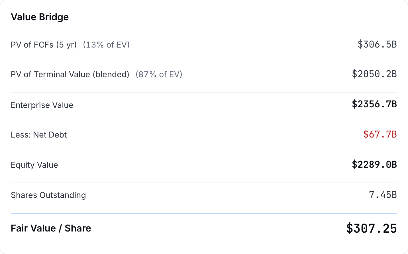
The figure below is the tab's own version of step 3, on the demo's Microsoft page. The bridge starts from the enterprise value the projection and the terminal value add up to, takes off net debt, and divides by the share count, and the last line is the fair value the headline tile shows.
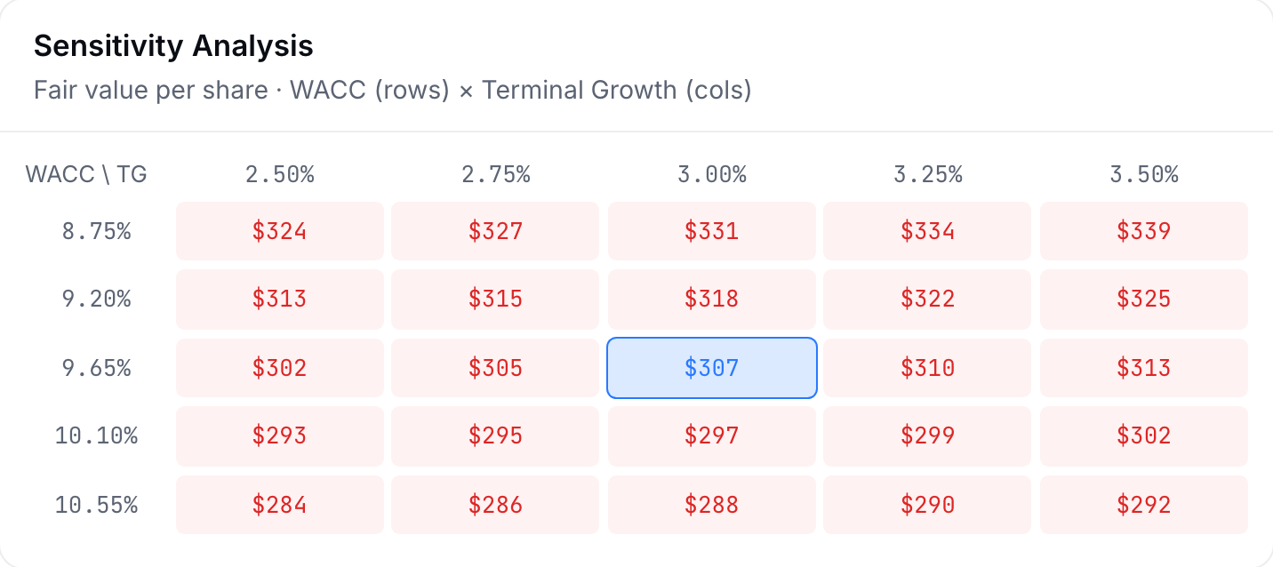
The second card on the tab is the one the rest of the chapter is about. It is a grid of twenty-five fair values, five discount rates down the side against five terminal growth rates across the top, in quarter-point steps, with the base case in the middle. The rows are made by moving the risk-free rate half a point at a time, which moves the WACC by a little less than that, since only the equity share of the capital structure feels it.
The widget below is a live version of that grid, built on the worked example. Nudge the terminal growth or the WACC and watch the fair value move, and notice how far it moves for a quarter point in either direction.
Having watched the number move, you should be able to say why the tab leads with the grid rather than with the single fair value. The question below asks you to.
Check yourself
Why does the DCF tab's headline output include a 5x5 sensitivity grid (WACC against terminal growth) instead of just the fair value?
- To look more professional in pitch decks. The grid does look sharp in a pitch deck, but that is a side effect rather than the reason it exists. The reason has to do with where the value in a DCF concentrates.
- Because fair value depends so heavily on the terminal assumptions, the grid is the right thing to report. (correct) Right. Recall that the worked example put 86% of the value in the terminal assumption. A single fair value hides that fragility from the reader, while the grid shows the range of fair values your uncertainty actually implies, and the methodology itself flags the DCF fair value as "sensitive to the analyst-set terminal assumptions".
- Because the model cannot converge to one number. The model converges to a single number just fine. The grid exists because that single number tells the reader quite a bit less than the twenty-five numbers taken together.
The check below puts a number on the same point, using the worked example's terminal value and moving the growth assumption by a single point.
Practice
In the worked example, recompute the terminal value with terminal growth at 3% instead of 2% (same WACC of 10%). Enter the new TV in $M.
Solution. 113.3 / 0.07 = $1,618.6M, compared with $1,402.5M when growth was 2%. Take a moment to think about the size of that move. One assumption moved by a single point and the terminal value changed by 15%, and nothing about the underlying business changed at all. This means that whoever sets the growth assumption controls a large share of the fair value. So the tab makes the sensitivity grid, and not the single number, its headline output.
Everything we have done so far has assumed, without saying so, a company that makes money, and a good number of the companies you will be asked to value do not. Imagine an electric truck maker that lost $3.6 billion from operations last year on revenue of $5.4 billion, which is an operating margin of about negative 67 percent. If we hand that margin to a model that applies one margin to all five projected years, the model will project five more years of the same losses and produce a fair value below zero, which is not a useful answer for anyone deciding whether to own the stock. The more useful question is how quickly the losses shrink and where the margin settles once the business reaches scale. So when the latest 10-K shows an operating loss, the "Seed from latest 10-K" button makes the reported margin the year 1 operating margin, and the projection moves in equal steps from there to the target operating margin you set for year 5.
Take a moment to notice what the seed does and does not do for you here. The filing can tell you where the company is today, but it cannot tell you where the margin ends up, so the target margin stays your input, and it is the number a committee will spend the most time asking you to defend. To help with the part the filing can answer, the seed card lists every line it read from the 10-K (total revenues, the operating loss and the rest) with the units the filing uses, which means that each input in your report can be cited back to the line it came from.
So far we have run the model forward, from assumptions to a value, but running it backward is often just as useful. A reverse DCF takes today's share price as given and asks what one assumption would have to be for the model's fair value to equal that price, with every other input held where you set it. In other words, instead of asking what the stock is worth, it asks what the market is already assuming when it pays the current price. On the tab this is a single line under the fair value (click it to open the full view), and it solves for two things separately, the operating margin the company would need to reach by year 5 and the revenue growth rate it would need to sustain for all five years.
The reason this helps is that it turns an argument about a fair value into an argument about a business. Suppose the line says the price assumes a 23 percent operating margin by year 5 while your model uses 15 percent. You and the market are then disagreeing about whether this company can earn a margin that few carmakers have ever reached, and that is a question you can take to the filings and to the peer margins on the Competitive Position tab. The question below checks which way that disagreement pushes your fair value.
Check yourself
The Reverse DCF line says the current price assumes a 23% operating margin by year 5, and your model uses 15%. Holding your other inputs where they are, where does your fair value sit relative to the price?
- Above the price, because a lower margin makes your model the more conservative one. This one has the potential to be tricky. A lower margin means less operating income and less cash flow in every projected year, which lowers the value, so your fair value comes out below the price rather than above it.
- Below the price, because the price needs a higher margin than you assume. (correct) Right. The price only makes sense with a 23% margin, and your model gives the company less than that, so your fair value lands below the price. This means that, in your model's view, the market is paying for more than you think the business will deliver.
- Equal to the price, since the reverse DCF solved for it. The reverse DCF solved for the margin that would make the two equal, but your model is still using 15%. Only if you moved your target margin up to 23% would your fair value meet the price.
Banks need a model of their own, because a bank's debt is the raw material of its business rather than a way of paying for it, which makes free cash flow a confusing figure to build a valuation on. The tab's Bank DDM values the dividends instead, discounting five years of them at the cost of equity (which starts at the CAPM figure from the bank's own beta) and adding a terminal value at the end. One leg of that terminal value prices the bank at a multiple of its book value, and rather than asking you to guess that multiple, the tab computes it from the bank's return on equity (ROE) with the justified price-to-book ratio.
The justified price-to-book
ROE is the return the bank earns on its book equity, CoE is the return its shareholders require, and g is the long-run growth rate of its dividends. The tab holds the result between 0.2x and 5x.
Take a minute to read the formula in words. If a bank earns exactly what its shareholders require (ROE equal to CoE), the top and the bottom of the fraction are the same and the ratio is 1, so a dollar of book equity is worth a dollar. A bank that earns more than its cost of equity is worth more than its book value, and one that earns less is worth less, which is why moving the ROE input on the tab moves the fair value. Let's compute one.
Practice
A bank earns a 15% return on equity, its cost of equity is 10%, and its dividends grow at 3% a year over the long run. Compute its justified price-to-book ratio.
Solution. 0.12 / 0.07 = 1.71x. Take a moment to think about what that means. Every dollar of this bank's book equity is worth about $1.71 to its shareholders, because the bank earns 15 cents on each dollar of equity while its shareholders only require 10. If the bank's ROE fell to 10%, the top of the fraction would match the bottom and the ratio would drop to 1. In other words, the bank would be worth its book value and no more.
The lab asks you to make one prediction before you touch anything, because if you can predict the direction and the rough size of a move before you make it, you understand the model rather than just operating it.
Lab: Lab: predict before you look
- Open Research, load a ticker you know, and open the DCF tab. Press "Seed from latest 10-K" so that the growth, margin, tax and conversion inputs start from reported financials rather than from the sector defaults. (The tab also has two alternate models for businesses a standard DCF handles badly, an Alt Manager model built on fee-related earnings and a Bank DDM.)
- Write down the base-case fair value. Then, before touching anything, predict which way fair value will move if you raise terminal growth one notch, and roughly by how much.
- Make the change and check your prediction against the sensitivity grid. One notch of the terminal growth slider is a quarter point, which is exactly one column of the grid, so the cell you land on was in the grid before you asked.
- Open the Reverse DCF line under the fair value and compare the operating margin the price assumes with your own target margin. Press its Try button to move your target to that margin and confirm that the fair value lands on the current price, then press Reset inputs to put every input back.
- Press Export CSV on the DCF tab and verify one year's discounting by hand. In the projection table, the FCF ($B) column divided by (1 + WACC)^year, with the WACC from the assumptions block at the top of the file, should match that year's PV ($B) column.
Sources
- Gordon, M. J., and Shapiro, E. (1956). Capital equipment analysis: The required rate of profit. Management Science, 3(1), 102-110 https://pubsonline.informs.org/doi/10.1287/mnsc.3.1.102
The Analyst's Handbook is Sifter's textbook for student investors, written by Matt Lang and Bree Lang. Sifter is free for students. This chapter as markdown.